Generative Adversarial Networks - Part V

This is the Part 5 of a short series of posts introducing and building generative adversarial networks, known as GANs.

In this post we'll learn about a different architecture called a conditional GAN which enables us to direct the GAN to produce images of a class that we want, rather than images of a random class.

Previously:

• Part 1 introduced the idea of adversarial learning and we started to build the machinery of a GAN implementation.
• Part 2 we extended our code to learn a simple 1-dimensional pattern 1010.
• Part 3 we developed our code to learn to generate 2-dimensional grey-scale images that look like handwritten digits
• Part 4 extended our code to learn full colour faces, and also developed convolutional networks to encourage learning localised image features

Controlling What A Gan Creates

In parts 3 and 4 of this series, we trained a GAN on data that contained unique and diverse images. Each handwritten digit in the MNIST dataset is different, and each face in the CelebA data set is unique.

When we use the trained generator to create an image, we have no control over what kind of image it creates. All we know is that the image will be plausible enough to get past the discriminator.

We can't ask the generator from part 3 to create a 7 or a 9 for us. All we can do is feed the generator a random vector of numbers as input and see what image pops out.

If we experiment with that random input, in an attempt to control what comes out of the generator, we find that it doesn't sufficient, if any, control over the output.

Is is possible to train the generator so that we can influence the output?

The answer is yes, and that is what a conditional GAN architecture aims to do.

Conditional GAN Architecture

The following picture shows the conditional GAN architecture.

You can see that both the generator and discriminator are provided with additional information about the image. For us, this additional information can be a label, such as the digit an MNIST image represents.

It is not immediately clear how this helps. Let's break it down:

• The discriminator can use the label to improve how it identifies whether an image is real or fake. How it does this is up to itself, additional information can only help. Without the label, the discriminator has a set amount of information on which to make the decision. With the label, it has additional information. 

• The generator can learn to associate the label with the image it generates. It doesn't have to - it could choose to ignore the additional information. But the generator learns by getting feedback from the discriminator, which has learned to associate the label with an image, so the generator is encouraged to make this association too by generating images that match the image-label pair the discriminator sees from the training set.

Training A Conditional GAN

The training loop is unchanged from a vanilla GAN. The only difference is the additional information appended to the inputs to the generator and the discriminator:

• The discriminator is shown a real image from the training dataset, as well as that image's label. It is trained to output a 1 for real.

• The discriminator is shown a fake image from the generator together with its label, and is trained to output a 0 for fake.

• The generator is trained to cause the discriminator to output a 1 for real.

The labels associated with the real images are part of the training data.

The labels associated with the generator are randomly chosen one-hot vectors of the same length as the labels in the training dataset. We just need to make sure that this randomly chosen label remains the same when fed into the generator as part of the seed, and when associated with the generated image for the discriminator to test. We can't have a different label for these two parts of the training.

When feeding the generator, the one-hot label vectors are combined with the random seed by concatenating the tensors like this:

def forward(self, noise_tensor, label_tensor):
    # combine image and label
    inputs = torch.cat((noise_tensor, label_tensor),1)
    
    # simply run model
    return self.model(inputs)

Similarly, when feeding the discriminator the one-hot label vectors are combined with the image data like this:

def forward(self, image_tensor, label_tensor):
        # combine image and label
        inputs = torch.cat((image_tensor.view(1, 784), label_tensor),1)
        
        # simply run model
        return self.model(inputs)

The following shows code for the training loop:

# train Discriminator and Generator

epochs = 12

for i in range(epochs):
    print('training epoch', i+1, "of", epochs)
    
    for label, image_data_tensor, target_tensor in mnist_dataset:
      
        # train discriminator on real data
        D.train(image_data_tensor.view(1, 1, 28, 28), target_tensor, torch.cuda.FloatTensor([1.0]).view(1,1))
        
        # random 1-hot label for generator
        random_target_tensor = generate_random_target(10)

        # train discriminator on false
        # use detach() so only D is updated, not G
        # label softening doesn't apply to 0 labels
        D.train(G.forward(generate_random(100).view(1,100), random_target_tensor).detach(), random_target_tensor, torch.cuda.FloatTensor([0.0]).view(1,1))
        
        # random 1-hot label for generator
        random_target_tensor = generate_random_target(10)
        
        # train generator
        G.train(D, generate_random(100).view(1,100), random_target_tensor, torch.cuda.FloatTensor([1.0]).view(1,1))
        
        pass
    
    pass

The full code is online:

• https://github.com/makeyourownalgorithmicart/makeyourownalgorithmicart/blob/master/blog/generative-adversarial-network/05_image_cgan_mnist.ipynb

Results

The results of training should be a generator that can create images of a desired class by providing it with the label as well as the normal random seed. So feeding the generator a label of 1 should result in images that look like a hand-drawn 1.

The following shows the results of 12 epochs of training.

The zeros at the top left are produced by feeding the trained generator a random seed augmented with a one-hot vector corresponding to the label 0, which would be 1000000000.

We can see that for each input label, the generator does indeed produce images of that label.

The following shows the results for 24 epochs of training:

The quality of the digits has improved.

As an experiment to see how important the labels are to training, the following set of results are from the same code but with the one-hot vector to the discriminator set to 0000000000.

We can see two things:

• the generator no longer creates images of the desired class
• the image quality overall is lower than without the label

This shows that it is important for the discriminator to learn the association between an image and its class, for it to then feed the generator useful gradients to learn from. The lower quality is likely a result of the fact that we have, in effect, an enlarged image to learn which means longer training time or perhaps a more efficient neural network design, referred to as the hyper-parameters.

Experimenting With Input Labels

Let's see what happens when we use input labels to the trained generator that are not 1-hot but have several elements activated?

We can use the plot_images() generator method to activate more than one location by supplying a tuple of labels. The following sets the input vector to be [0, 0, 0, 0, 0, 0, 1, 0, 0, 1].

G.plot_images((6,9))

The resulting images are shapes which are intermediate between 6 and 9.

This is interesting as it shows that we can manipulate the input vector in ways that have a visual meaning.

The following shows the results for G.plot_images((3, 5)).

That also broadly works. Let's try a more challenging combination, G.plot_images((1, 7)).

The results are understandable as it is hard to find a shape that is both 1 and 7 in nature.

Conclusion

If we think about these results, they're quite impressive.

We've managed to not only to train a GAN to generate plausible images, where the generator has not directly seen the training data, we've also managed to control the class of image being generated by associating the learned representation with a label we provide.

Previously the learned representation was entangled, and it was difficult to induce the generator to produce an image of the class we wanted just by manipulating the random seed.

We also saw how we can manipulate the input vector to create images which have shapes representing combinations of more than one class. 

More Reading

• Good explanation and discussion in this paper, Conditional Generative Adversarial Nets For Convolutional Face Generation: http://www.foldl.me/uploads/papers/tr-cgans.pdf (pdf)

• The (original?) paper on conditional GANs: https://arxiv.org/pdf/1411.1784.pdf (pdf)

Generative Adversarial Networks - Part IV

This is the Part 4 of a short series of posts introducing and building generative adversarial networks, known as GANs.

Previously:

• Part 1 introduced the idea of adversarial learning and we started to build the machinery of a GAN implementation.
• Part 2 we extended our code to learn a simple 1-dimensional pattern 1010.
• Part 3 we developed our code to learn to generate 2-dimensional grey-scale images that look like handwritten digits

In this post we'll extend our code again to lean to generate full-colour images, learning from a dataset of celebrity face photos. The ideas should be the same, and the code shouldn't need much new added to it.

Celebrity Faces

A popular dataset for human faces is the celebA dataset which contains 202,599 photos, annotated with some features.

A revised version was developed, called the aligned celebA dataset, where the location of the eyes is consistent across the dataset and the orientation of the heads is vertical so the mouth is below the eyes were possible. The following shows 6 samples from the dataset.

From a code perspective, it is cumbersome to use a folder of over 200,000 images. It is much easier to work with a data structure which contains the images as numerical arrays.

The terms of use prevent me sharing this repackaged dataset, but the following snippet of code will convert the provided zip into a hdf5 file.

• github gist: celeba_zip_to_h5py

HDF5 is a format designed to store large amounts of data for efficient access and processing in a portable manner. Python's pickle approach is not as scalable, and has additional security concerns.

The following code illustrates how to use the python h5py library to extract images from this hdf5 file:

import h5py

with h5py.File('my_data/My Drive/Colab Notebooks/gan/celeba_dataset/celeba_aligned_small.h5py', 'r') as file_handle:
  dataset = file_handle['img_align_celeba']
  image = numpy.array(dataset['000007.jpg'])
  plt.imshow(image, interpolation='none')
)

You can see that a hdf5 file is opened just like a normal file. As the hdf5 format is hierarchical, we first select which dataset we're interested in, here img_align_celeba. That gives is a dictionary-like structure where the keys are the image file names. Here we pick 000007.jpg and convert the returned data into a numpy array before plotting it.

The image data is of the form (height, width, 3) where the 3 is required for the red, green and blue colour values.

Simple Discriminator and Generator

Following our philosophy of starting small and simple, we'll see how well a very simple discriminator and generator made of a single hidden layer of fully connected nodes works.

The following is a simple discriminator model consisting of an input layer of size 3*218*178 = 116412 nodes, a hidden layer of 100 nodes, and a final output layer of 1 node which is sufficient for a 1 (true) and 0 (false) output.

# define neural network layers
# input shape is (1, 3, height, width)
self.model = nn.Sequential(
            
    View((1,3*218*178)),
            
    nn.Linear(3*218*178, 100),
    nn.LeakyReLU(),
        
    nn.LayerNorm(100),
            
    nn.Linear(100, 1),
    nn.Sigmoid()
)
        
# create error function
self.error_function = torch.nn.BCELoss()

# create optimiser, using simple stochastic gradient descent
self.optimiser = torch.optim.Adam(self.parameters(), lr=0.0001)

The incoming data is reshaped using View() to be 1-dimensional so it can be considered a single input layer of nodes. We're using the leaky relu and layer normalisation for the middle layer as we previously found that to be beneficial for GAN training.

As before, let's first check this network has the capacity to learn to discriminate between real data and random noise. If it can't even do that then it is intuitive that it can't tell the difference between images from the training set and images from the generator.

The core code for training the discriminator is as follows:

for image_data_tensor in celeba_dataset:
        
    # train discriminator on real data
    D.train(image_data_tensor.permute(2,0,1).contiguous().view(1, 3, 218, 178), torch.cuda.FloatTensor([1.0]).view(1,1))
    
    # train discriminator on false (random) data
    D.train(generate_random(3*218*178).view((1, 3, 218*178)), torch.cuda.FloatTensor([0.0]).view(1,1))
    
    pass

The code looks a little complicated so let's take it step by step. The data from the celeba dataset is of the form (height, width, 3). This needs to be reshaped to (1, 3, height, width), the 4-dimensional tensor expected by pytorch. The first 1 is a batch size. The permute() function re-arranges the axes and contiguous() is needed to repack the tensor as permute can cause the memory layout to become non-contiguous.

Similarly, the generate_random() creates a 1-dimensional array of random numbers, which we need to reshape to (1, 3, height, width).

As we're developing code, I've only taken 19,999 images from the 202,599 for the hdf5 file. The following shows the loss as the discriminator is trained once on this data.

We can see the loss falls to zero as training proceeds. It is interesting that a large number of the losses seem to be concentrated on a tight path.

Manually testing the trained discriminator shows it has been trained successfully.

We can now proceed to defining the generator. Again, let's keep its architecture as simple as possible.

# define neural network layers
# input shape is 1-dimensional array
self.model = nn.Sequential(

    nn.Linear(100, 3*10*10),
    nn.LeakyReLU(),

    nn.LayerNorm(3*10*10),

    nn.Linear(3*10*10, 3*218*178),
    nn.Sigmoid(),

    View((1, 3, 218, 178))
)

# create error function
self.error_function = torch.nn.BCELoss()

# create optimiser, using simple stochastic gradient descent
self.optimiser = torch.optim.Adam(self.parameters(), lr=0.0001)

As before, the generator takes a random input, in this case a 1-dimensional array of size 100. We use a middle layer of size 3*10*10 = 300 and again use the leaky rely and layer normalisation. The final layer grows to 3*218*178 which is the number needed for an image of size 218 by 178 and 3 red, green and blue channels.

The code to train the generator follows the same pattern as before - we train the discriminator to label real images as 1, images from the generator as 0, and we train the generator to get the discriminator to label its images as 1.

for image_data_tensor in celeba_dataset:
      
    # train discriminator on real data
    D.train(image_data_tensor.permute(2,0,1).contiguous().view(1, 3, 218, 178), torch.cuda.FloatTensor([1.0]).view(1,1))
    
    # train discriminator on false
    # use detach() so only D is updated, not G
    # label softening doesn't apply to 0 labels
    D.train(G.forward(generate_random(100)).detach(), torch.cuda.FloatTensor([0.0]).view(1,1))
    
    # train generator
    G.train(D, generate_random(100), torch.cuda.FloatTensor([1.0]).view(1,1))
    
    pass

Here are the results from one epoch through the dataset of 19,999 images.

Yippee!

Our GAN did actually learn to create faces. That's pretty amazing - especially when we remember the generator has not directly seen any of the celebrity photos.

Another nice thing is that the faces are different - so we've avoided mode collapse. The variety of images is really good - we can see both male and female faces, as well as different styles of hair a shapes for eyes and heads.

We can see the losses from the discriminator and the generator stabilise which suggests an equilibrium has been reached, which is good. Equilibrium in GAN training is sometimes hard to achieve, and a lack of it can lead to a collapse in useful training of the generator.

For a first attempt, these results are great.

The images were a bit grainy so let's see what a second training round does.

The images have improved significantly. The equilibrium between the discriminator and generator is holding.

Let's continue to more training epochs. The following shows the results for 4 epochs.

The results are improving, albeit we still have some of the grain. It is good to see the diversity maintained with different hair colour and even one oblique pose. This means we've avoided mode collapse.

Continuing to 6 epochs gives slightly improved images again.

The lower middle image is starting to show over-saturation which could be a sign we're reaching the limit of this training session.

At 8 training epochs we're starting to see both an improvement in some of the generated faces but also over-saturated blotching, and also some mode collapse. Two pairs of the images in the apparently random set above are very similar.

The loss charts are starting to show instability, which corresponds with this worsening of the generator.

The code for this simple GAN is online, and includes instructions to take advantage of a cuda gpu through google's hosted colab notebook service:

• https://github.com/makeyourownalgorithmicart/makeyourownalgorithmicart/blob/master/blog/generative-adversarial-network/04_celeba_gan.ipynb

The animation at the top of this blog is the output of the generator as the input array is varied in a controlled by, moving a set of consecutive 1's along the 100 length array in steps of 5, with the resulting images smoothly transitioned for effect.

Experiments - Change Size of Random Input

What we've developed is an intentionally simple architecture to get us started. We can do many experiments varying different elements of the networks design and architecture to see if they result in an improvement or not.

A simple experiment is to change the size of the random number array that feeds the generator. So far we've been using a size of 100. That number is effectively the first layer of the generator network. If it is too large, it makes training the generator harder. If it is too small, it may limit the variety of images the generator can create.

Here are the images resulting from 4 epochs of training, with the input array size varying as 5, 10, 100 and 200.

Overall the quality of the images doesn't change much. For very small input sizes, the image quality is poor, but actually surprising good. Having an input of size 1 into the generator still creates diverse images that do look like faces, even if the quality is poor and there is mode collapse.

The quality seems to improve slowly as that input size grows. At size 400, the images are diverse and contain different features but are starting to look like they need more training. This is expected, because larger networks take longer to train.

The only slight surprise here is that an input of 1 random number into the generator still results in faces being generated.

Convolutions for Selecting Features

A very common improvement in GANs, and indeed neural networks more generally, is the use of convolution layers. Instead of connecting every input node to every node in the next layer, we can limit the connections to a smaller area of the input. This means the next layer picks out local features of the input.

The following diagram (src) shows how a convolution kernel K picks out diagonal features from an image I. The feature map S has a high value of 1 in the bottom right because the original image has a diagonal pattern in the bottom right. Similarly, the top right has no diagonal pattern and that's why S has a 0 there. Partial patterns in the image, such as the top left, result in partial values in S.

The following notebook implements a simple classifier neural network for the handwritten digits dataset from part 3, and shows that learning localised image features results in the accuracy jumping from 90% to 98%:

• https://github.com/makeyourownalgorithmicart/makeyourownalgorithmicart/blob/master/blog/generative-adversarial-network/02_mnist_pytorch_cnn.ipynb

The following animation (src) shows how a convolution reduces the size of the image to a smaller feature map:

You can see how this locally limited passing of information from the input (blue) to the next layer (green) can allow image features to be learned. For this reason convolution layers are popular for classifying neural networks - and in our work, the discriminator.

For the generator, we can use convolutions again but they need to work in the opposite direction. Instead of shrinking the input, we need the generator to expand the input noise array towards the size of the output image. These are called transposed convolutions, or sometimes deconvolutions.

It is worth noting that generators are often designed to be similar to their discriminator but reversed in direction. There is no real reason to do this, other than as a loose heuristic approach to balancing the generator and discriminator.

The following animation (src) shows this working. The 3x3 input (blue) is expanded to the 5x5 output.

Initial experiments failed to produce results. Here's an early experiment.

The striping or moire-like pattern problem is common when trying to build images from inverse convolutions. This is because they can overlap if not spaced apart just right. This is achieved my making sure the stride or step size divides the size of the kernel.

Here is another example which failed to generate celebrity faces, but did succeed in creating monsters from some horror film!

After much experimentation I did find a working, and still simple, solution.

The following shows how the generator and the discriminator are broadly balanced. The images themselves have been cropped to be a square 128x128 because the inverse convolutions are much easier to design to have an output that is 128x128 and avoid having a linear layer at the end of the generator.

The discriminator has three convolution layer with kernels of size 8, which move in steps of 2. After the convolutions have reduced the input to a 3x10x310 feature map, a linear layer reduces these 300 values down to 1.

self.model = nn.Sequential(
    
    nn.Conv2d(3, 256, kernel_size=8, stride=2, bias=False),
    nn.BatchNorm2d(256),
    nn.LeakyReLU(0.2),
    nn.Dropout2d(0.3),
    
    nn.Conv2d(256, 256, kernel_size=8, stride=2, bias=False),
    nn.BatchNorm2d(256),
    nn.LeakyReLU(0.2),
    nn.Dropout2d(0.3),
        
    nn.Conv2d(256, 3, kernel_size=8, stride=2, bias=False),
    nn.LeakyReLU(0.2),
    nn.Dropout2d(0.3),
 
    View((1,3*10*10)),
        
    nn.Linear(3*10*10, 1),
    nn.Sigmoid()
)

We are also expanding the 3 channels to 256 for the convolutions, which is simply having 256 different potential feature selectors at each layer. This gives the network a larger capacity to learn more potentially useful features.

This discriminator also has dropout. This means that some of the network signals are zeroed during training, which helps avoid overfitting by preventing nodes from co-adapting.

Testing the discriminator by training it to separate real images from random noise shows that it does learn very well. The loss plot shows an interesting residual loss but the bulk of loss values fall towards zero.

Manually testing the discriminator shows very confident scores. This again confirms the general belief that convolution neural networks are better at image classification because they learn meaningful features.

The following is code for the generator. It is a bit smaller than the discriminator because there are only two convolution layers. Researchers are finding that in a balanced architecture, generators can be a bit smaller than the discriminators.

self.model = nn.Sequential(
            
    # input is a 1d array
    nn.Linear(100, 3*28*28),
    nn.LeakyReLU(0.2),
    
    # reshape to 2d
    View((1, 3, 28, 28)),
     
    nn.ConvTranspose2d(3, 256, kernel_size=8, stride=2, bias=False),
    nn.BatchNorm2d(256),
    nn.LeakyReLU(0.2),
            
    nn.ConvTranspose2d(256, 3, kernel_size=8, stride=2, padding=1, bias=False),
    nn.BatchNorm2d(3),
    nn.LeakyReLU(0.2),
               
    View((1,3,128,128)),
    nn.Tanh()
)

Here are the results from 1 epoch of training:

These aren't photo-realistic portraits but the results are impressive because we've succeeded, even with very simple code, in constructing images from localised features, as learned by the convolution layers. These features are, in effect, the eyes, nose, hair, lips, and so on. Looking closely we can see the patching together of these features.

Also impressive is he diversity of the images, each generated by a random input to the generator. We've avoided mode collapse.

Here are the results from 2 epochs:

Here are the results from 4 epochs:

As training progresses, the composition of faces improves. Each of the faces does have two eyes, a mouth and a nose, with hair in roughly the right place. We do see mismatched eyes and hair.

Here are the results from 6 epochs:

Here are the results from 8 epochs:

Again, the quality of the faces is improving, with the patching becoming smoother.

Here are the results from 10 epochs:

Here are the results from 12 epochs:

Each of these training epochs took about half an hour using colab, and it would be interesting to continue the training for more epochs, and also use the full dataset of 200,000 images and not the smaller 20,000 used for these experiments.

There is a loss of contrast as the training progresses which I haven't yet understood. The geometric features are the primary means of getting past the discriminator. The relative strengths of colours, the contrast, might not be learned by the feature based discriminator.

The following shows a selection of generated images, animated using a smooth transition.

The final code is online:

• https://github.com/makeyourownalgorithmicart/makeyourownalgorithmicart/blob/master/blog/generative-adversarial-network/04_celeba_gan_conv.ipynb

Tips and Heuristics

The theory that underpins GANs is still being developed and for this reason the design and training is too often unsuccessful or not efficient.

Researchers have mostly coalesced around a few heuristics and tips, mostly derived from experience and empirical results:

• Gaussian weight initialisation can help, just as it seems to help some traditional classification networks.

• For GANs, convolution kernel sizes should be larger than the 3x3 or 4x4 often found in textbooks. Our own example uses 8x8 kernels.

• Using a stride that exactly divides the size of the deconvolution kernel can avoid striping or moire-like patterns.

• Avoid normalising the last generator and first discriminator layers. The explanation offered is that this ensures the network can learn the actual mean and variance of images. 

• Square images are much easier to work with when trying to get inverse convolutions to produce images that are the size we want.
• Avoid overconfidence in the discriminator by training it to target 0.9 instead of 1.0 which can lead to gradient saturation, and so slow or no learning. This is called soft-labelling. That 0.9 can be varied by small random amounts.

• Occasionally flipping the true/false training target values helps the networks get kicked out of local-minima or periods of low-gradients.

• Normalising the data to the range -1 to +1 helps it match the activation functions where they have the best gradients for learning. 

Published Results

The following is an example of the current state of the art (src):

What does it take to produce these images?

The linked paper shows the hardware and training times:

Each GPU costs about £8,000 and 8 of them were used, with training times extending into days if not weeks!

Talk at Algorithmic Art June 2019

I gave a talk on this journey at the June 2019 meeting of the Algorithmic Art group.

A video recording is here: https://skillsmatter.com/skillscasts/13999-algorithmic-art-june-meetup

Slides for the talk are here: https://tinyurl.com/y3n55acf

Conclusion

The adversarial approach for training competing learning models is a markedly different idea to the large bulk of machine learning.

The theoretical underpinning is still being developed, and so for now not all architectures work well - with notable problems like mode collapse.

Even so, the results possible from very simple, as well as the very expensive state of the art, are impressive.

The future of generative adversarial machine learning is looks very promising!

More Reading

• You can find more visualisations of convolution and deconvolution here: https://github.com/vdumoulin/conv_arithmetic
• Dropout: http://jmlr.org/papers/volume15/srivastava14a/srivastava14a.pdf 
• Ian Goodfellow's seminal paper on GANs: https://arxiv.org/pdf/1406.2661.pdf
• Ian Goodfellow's tutorial paper on GANs including ideas for improving performance: https://arxiv.org/pdf/1701.00160.pdf
• Google's own GAN tutorial on colab: https://colab.research.google.com/github/tensorflow/docs/blob/master/site/en/r2/tutorials/generative/dcgan.ipynb 
• PyTorch's DCGAN tutorial: https://pytorch.org/tutorials/beginner/dcgan_faces_tutorial.html
• Using Google's colab service: https://medium.com/@oribarel/getting-the-most-out-of-your-google-colab-2b0585f82403
• Oreilley's GAN tutorial using tensforflow: https://github.com/dmonn/dcgan-oreilly/blob/master/DCGANs%20with%20Tensorflow.ipynb

Generative Adversarial Networks - Part III

This is the Part 3 of a short series of posts introducing and building generative adversarial networks, known as GANs.

Previously:

• Part 1 introduced the idea of adversarial learning and we started to build the machinery of a GAN implementation.
• Part 2 we extended our code to learn a simple 1-dimensional pattern 1010.

In this post we'll develop our GAN further to to learn, not a single pattern, but a collection of patterns. We'll also start to see some of the difficulties of training a GAN, which we'll try to address in the next post.

In this post I won't focus too much in PyTorch as that will distract us from exploring the ideas. The PyTorch code is essentially the same as what we developed previously, with the only differences being relatively boring details like how to load the training data and display 2-dimensional images. All the code will be provided on github for you to examine.

MNIST Dataset of Handwritten Digits

The patterns our GAN will be learning to generate are hand written digits 0-9. There is a very well known and used dataset called MNIST. It contains 60,000 images intended for training and 10,000 intended for testing. The images are 28x28 pixels in size, and are provided with the correct labels.

You can read more about how to get and understand the dataset here: link.


Big Picture
Before we dive into coding let's draw a big picture view of our GAN architecture.

There are one key difference from our previous GAN. The training data is no longer a single 1-dimensional pattern 1010, but is a collection of 2-dimensional images. Each image in the training dataset is different to any other one.

The other differences are just extensions from 1-dimensional data to 2-dimensional data. For example, the output of the generator is a 28x28 image, just like the training data. The discriminator now accepts a 2-dimensional 28x28 image, but still outputs 1 for real and 0 for fake.

With the overview in our minds, let's work through each section, step by step.

Discriminator

The job of the discriminator is to successfully distinguish between images from the real training data set, and images coming from the generator.

The question for us is what architecture, size and shape should the discriminator have? Should it have many layers? Should it use convolutions or the traditional fully connected nodes? What activation function should we use? How big should the layers be?

There isn't a perfect answer to this question. In fact, deciding exactly what network architecture is suitable for a task is an open research question.

A good approach for us is to start with a small simple neural network and check that it can first learn to classify the MNIST dataset. If a smaller network works for us, then we don't want a larger one that will be harder to train, require more computational resource and risks behaving in unexpected and unwanted ways.

The loose rationale is that if our small network can learn to classify MNIST data against the 10 labels, then it should have enough capacity to perform the simpler task of classifying against 2 labels real/false.

Let's start with very simple classifying network:

• Input layer of 784 nodes to match the 32x32 image pixels.
• Hidden middle layer of 200 nodes, with a simple sigmoid activation.
• Output layer of 10 nodes, one for each class 0-9, with a simple sigmoid activation to match the desired 0-1 output range.
• Binary cross entropy loss (BCELoss) as it penalises incorrect classifications stronger than the vanilla mean squared error loss (MSELoss).  
• Simple stochastic gradient descent (SGD) rather than anything fancy like Adam.

The code that implements this simple architecture is:

# define neural network layers
self.model = nn.Sequential(
    nn.Linear(784, 200),
    nn.Sigmoid(),
    nn.Linear(200, 10),
    nn.Sigmoid()
)
        
# create error function
self.error_function = torch.nn.BCELoss()

# create optimiser, using simple stochastic gradient descent
self.optimiser = torch.optim.SGD(self.parameters(), lr=0.01)

Training this classifier on the 60,000 training images and testing it on the 10,000 test images gives a very respectable 90% accuracy. Not bad for a very simple network.

The following shows the classifier loss as training progresses for 3 epochs.

And the following shows a manual check to see if an image is correctly classified. We can see the confidence in the label 2 is high.

You can see the full code for this MNIST classifier online:

• https://github.com/makeyourownalgorithmicart/makeyourownalgorithmicart/blob/master/blog/generative-adversarial-network/02_mnist_pytorch.ipynb

This confirms this simple network can learn to classify MNIST so we can reasonably assume it has the capacity to learn the simpler task of discriminating between real and generated images.

The discriminator network only has one output so the last layer is changed to have just 1 output node.

# define neural network layers
self.model = nn.Sequential(
    nn.Linear(784, 200),
    nn.Sigmoid(),
    nn.Linear(200, 1),
    nn.Sigmoid()
)

Couldn't be much simpler!

Is there any way can gain some confidence this discriminator can work with a single node output, beyond the reasonable argument we just made? Yes - we can train it to output 1 when seeing real images, and output 0 when seeing random noise.

The following shows the discriminator loss getting smaller when trained on real images and random noise. While we're developing the code, we'll use the smaller 10,000 training set rather than the larger 60,000 training set.

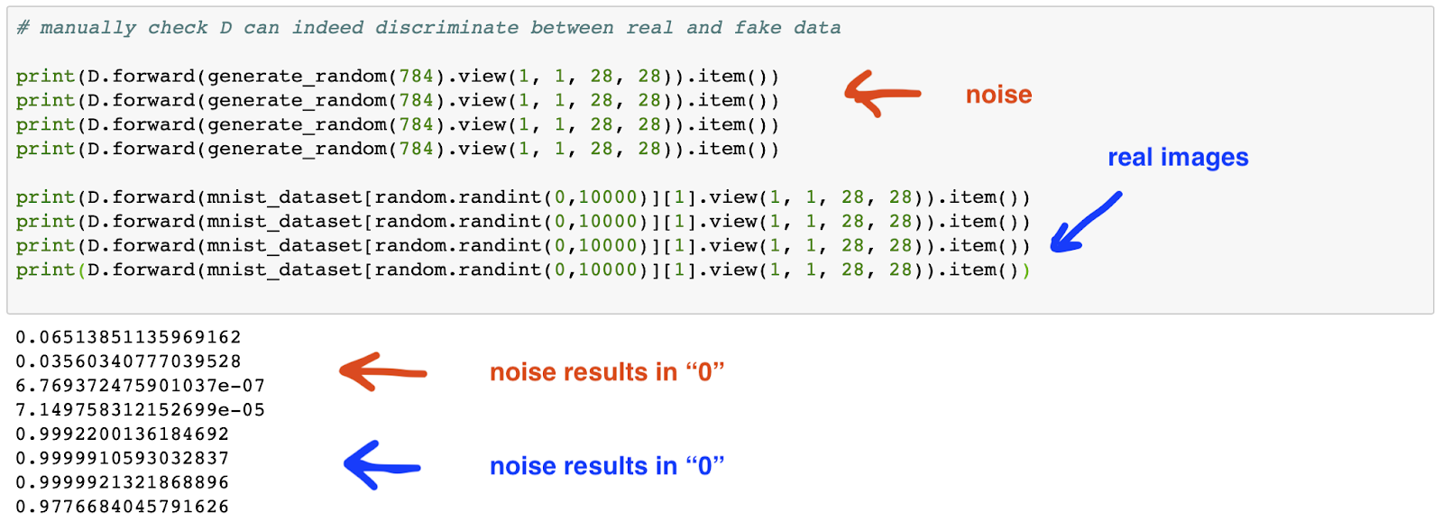
Let's manually test the discriminator with real image and random inputs.

The discriminator seems to be capable of learning the difference between real images and noise, which although not an ideal test of its capability, provides some confidence that we can include it in the GAN.

Generator

The generator needs to take random noise as input and output a 28x28 image. There are two questions that we need to answer:

• what size of random noise array should we use?
• what kind of neural network do we need between the input and output layers?

On the first question, there isn't an analytic answer we'll have to use an educated guess. Too small an input and we make it hard for the generator to provide a diverse set of output images. Too large and we waste computational resource, making the network hard to train. Given the output image has 28*28 = 784 a good starting guess is 100.

On the second question we should follow our previous approach of starting as small as possible and only growing the size and complexity if needed. If we only had one hidden layer, what size should it be? If the output is 784 nodes, this hidden layer needs to provide the network with the capacity to learn different images. This suggests a size of larger than 784, but let's see if we can get a smaller 500 to work.

So let's start with a generator network with the following:

• Input layer of 100 nodes to receive the random noise.
• Hidden middle layer of 500 nodes, with a simple sigmoid activation.
• Output layer of 784 nodes to form 28x28 images, with a simple sigmoid to match the target 0-1 range.
• The same simple BCE loss and SGD gradient descent methods as the discriminator. 

The following code is is the model for generator:

# define neural network layers
self.model = nn.Sequential(
    View((1,100)),

    nn.Linear(100, 500),
    nn.Sigmoid(),
    
    nn.Linear(500, 784),
    nn.Sigmoid(),
            
    View((1,1,28,28))
)

Again, very simple.

Let's remind ourselves of the training process. The following steps are repeated for all the training images:

• train the discriminator on a real image with a target output of 1.0 (true)
• train the discriminator on a generated image with a target output of 0.0 (false)
• train the generator to cause the discriminator to produce a 1.0 (true)

The training code looks like this:

# train Discriminator and Generator

epochs = 1

for i in range(epochs):
    print('training epoch', i+1, "of", epochs)
    
    for label, image_data_tensor, target_tensor in mnist_dataset:
      
        # train discriminator on real data
        D.train(image_data_tensor.view(1, 1, 28, 28), torch.FloatTensor([1.0]).view(1,1))

        # train discriminator on false
        # use detach() so only D is updated, not G
        D.train(G.forward(generate_random(100).view(1, 1, 10, 10)).detach(), torch.FloatTensor([0.0]).view(1,1))
        
        # train generator
        G.train(D, generate_random(100).view(1, 1, 10, 10), torch.FloatTensor([1.0]).view(1,1))
        
        pass
    
    pass

You can see an outer loop which allows the training to be repeated for a given number of epochs.

Using the smaller 10,000 training set, the discriminator loss looks like this:

The loss fall quickly as the discriminator learns to tell real and generated images apart. Remember, in the early stages, the generator will not be creating good images, and the discriminator will find it easy to tell them apart from the real images. As training continues the generator gets better, the discriminator seems to get worse again, but towards the end approaches a loss of 0.5 which is the theoretical equilibrium when it can't tell real and generated images apart.

The generator loss - or more accurately the discriminator loss caused generated images - rises as training progresses because it gets better at fooling the discriminator.

Let's see a sample of six generated images after one round of training - 1 epoch.

There's good news and bad. The good news is that the images are not random noise and have some kind of structure in the middle of the area. The bad news is that the structures aren't recognisable as digits.

Let's run another round of training.

We can see the discriminator loss falls below 0.5 and the generator loss rises. The resulting images are all similar and very spiky (high contrast). What appears to have happened is that the generator has found a solution that is very good at fooling the discriminator.

Let's try four more rounds of training so we have a total of 6 epochs.

That hasn't improved the results. The generator is producing even more spiky images. The high contrast which means it has high confidence that they will fool the discriminator.

The two problems we have are:

• the generator creates the same/similar images from different random inputs
• the images don't look like digits

The problem of a generator learning only one pattern, albeit a pattern that does fool the discriminator. The problem of the generator overwhelming the discriminator so the loss isn't balanced around 0.5 is because we've not reached an equilibrium between the adversarial discriminator and generator.

The code for this initial attempt at an image generating GAN is online:

• https://github.com/makeyourownalgorithmicart/makeyourownalgorithmicart/blob/master/blog/generative-adversarial-network/03_image_gan_first_attempt.ipynb

GANS Are Hard To Train

We've just seen how GAN training can partially fail.  The generator and discriminator were learning, but the state they ended up in wasn't what we wanted. We wanted the generator to be able to produce a range of images that look like digits.

Compared to normal neural network architectures, GANs are still a relatively new idea and the methods for training them are aren't yet fully understood. It is an active area of research.

It is possible for GAN training to totally fail with no convergence happening at all. We were lucky our simple network didn't see that.

If we can get our GANs to converge, the main issue is the generator not producing a range of images, like we saw earlier. Have a look at the following diagram from this paper (pdf).

The diagram shows real data which can be one of 8 different types. For example, we might have images of digits that are just 0-7. The diagram also shows a trained generator only producing images that match one of the 8 types. This is called mode collapse - the generator has found one solution that works and has fallen into it, and is unable to find other solutions that also work.

So how do we fix this?

Most of the current advice for turning GANs is heuristic or based on educate guesses. You'll find some of the suggestions apparently based on theory contradict each other. Some of the improvements suggested are architectural - even using several generators, instead of one.

There can be several causes of mode collapse, or even non-convergence. Here are some:

• a mismatch between the discriminator and generator - the adversarial game only works if both improve and one doesn't leave the other behind
• unbalanced training data (the MNIST training data is balanced)
• learning algorithms that suffer saturation or diminished gradients just like normal neural networks

Let's see if we can make small adjustments that fix this mode collapse.

Improving Training Updates

One of the most common changes made to GAN neural networks is the method by which the errors are used to update the network weights.

The basic stochastic gradient descent (SGD) is fine in many cases. It is also simple and fast, both of which are merits. One of its disadvantages is that it can jump about the error minimum that it is trying to get to as it isn't the best at adapting its weight change steps.

There are more sophisticated methods like the very popular Adam (adaptive momentum estimation) which has two key features:

• it has individual learning rates for each parameter, not one general learning rate
• the individual learning rates are adapted based on recent changes (momentum)

A very good explanation of Adam is here:

• https://machinelearningmastery.com/adam-optimization-algorithm-for-deep-learning/

The code change to use Adam is very simple. Note with Adam we typically use much smaller learning rates compared to SGD.

# create optimiser, using simple stochastic gradient descent
self.optimiser = torch.optim.Adam(self.parameters(), lr=0.0001)

A second improvement is within the neural networks themselves. The logistic activation function is simple and was historically popular. However, one of its major weaknesses is vanishing gradients for much if its input range. You can see this in the following graph. Gradients are needed for the update process, and if the network becomes saturated, or just has large values passing through it, then diminished gradients severely limit learning.

A very good answer is to use the rectified linear unit ReLU, or an improved version of it called a LeakyReLU.

The gradient on the right hand side remains strong. The small gradient on the left avoid the zero gradient problem leading to "dead ReLUs".

One more change that is also very common is to add normalisation layers into the network. A simple variant, called LayerNorm in PyTorch, is to take all the signals out of a network layer and normalise them so they they are centred about 0 and have a standard deviation of 1.

The following shows the updated discriminator:

# create optimiser, using simple stochastic gradient descent
# define neural network layers
self.model = nn.Sequential(
    ((1, 784)),
    nn.Linear(784, 200),
    nn.LeakyReLU(),

    nn.LayerNorm(200),
            
    nn.Linear(200, 1),
    nn.Sigmoid()
)

And the following is the updated generator:

# define neural network layers
self.model = nn.Sequential(
    View((1,100)),
            
    nn.Linear(100, 500),
    nn.LeakyReLU(0.2),
            
    nn.LayerNorm(500),
            
    nn.Linear(500, 784),
    nn.Sigmoid(),
            
    View((1,1,28,28))
)

Let's see if these improvements actually result in better generated images.

Here are the results from one round of training on the smaller 10,000 test set.

We can see the images from the generator now starting to look like real numbers. There are some that look like a 3 and some that could be a 9, or the beginnings of a 7 or a 1.

The discriminator loss follows a different pattern. The loss falls very rapidly due to the improvements we've made. However after a while, the losses start to increase as the generator starts to learns how to fool it. If you look closely, the losses in the discriminator caused by the generator are large.

Let's run the training again for a second epoch.

The digits are improving. The discriminator loss is still mostly low but with more samples being pulled upwards. We can see how over time the average might approach the theoretical 0.5.

Let's see what 4 epochs does:

This is a mixed picture. We have some digits much better defined like the 5 and 3, but some that are degrading.

And here's the result of 8 epochs.

Some, but not all, of the generated images are starting to look really good now.

The following is the result of 2 epochs training on the bigger 60,000 MNIST training set.

That's a much better result. The benefit is not just from the larger number of training examples, but the fact that they are different. Multiple epochs on a smaller dataset means repeating the same, and so less diverse, set of images.

You can explore the GAN code which includes these improvements here:

• https://github.com/makeyourownalgorithmicart/makeyourownalgorithmicart/blob/master/blog/generative-adversarial-network/03_image_gan.ipynb

Discussion

We've succeeded in training our generator to create images that look very like hand-written digits. And we did this while keeping our GAN neural networks very simple. We didn't need to have lots of layers or have more complex schemes like convolution layers.

We did experience the mode-collapse issue and overcame it with a stronger Adam optimiser, using the ReLU activation and the layer normalisation to help stabilise learning.

It is easy to understand how these improvements improve GAN convergence, but it is not immediately clear how these improvements, which apply to both the generator and discriminator, help avoid mode collapse.

The following chart shows the results of using combinations of Adam, layer normalisation and the ReLU activation, using 4 epochs of training on the smaller 10,000 MNIST test set.

Although not rigorous, these initial experiments suggest that the best results are from all three optimisations applied together. Individually, Adam on its own has the least benefit and seems not to break the mode collapse. LeakyReLU and layer normalisation break mode collapse. It's not overly clear but I think LeakyReLU has the most benefit.

In the next Part 4 of this series we'll try to learn more photo-realistic colour images, where we might have to expand our networks to use convolution and de-convolutions to learn localised image features.

More Reading

• Excellent overview of gradient descent methods: http://ruder.io/optimizing-gradient-descent/
• A short accessible video on GANs: https://www.youtube.com/watch?v=hQv8FNaJHEA
• In-depth tutorial by Ian Goodfellow: https://arxiv.org/abs/1701.00160