
Why? Prime Numbers.
Of all the things we can visualise, why this function?The motivation goes back to the mystery of prime numbers. Prime numbers are whole numbers which aren't the result of multiplying two other whole numbers. Here are some examples of numbers that are and aren't prime:
- 10 isn't a prime number because 10 is 5 times 2.
- 7 is a prime number, because we can't find two whole numbers that multiply together to give 7.
- 12 is not a prime number. There are several ways to make 12. For example, $12 = 4 \times 3$, and $12 = 6 \times 2$, and even $12 = 2 \times 2 \times 3$.
- The first few prime numbers are 2, 3, 5, 7, 11, 13, 17, 19, 23, 29, 31, 37, 41, 43, 47, ...
The idea of prime numbers is simple and many school children know what they are.
Despite that simplicity, the prime numbers have fiercely resisted a deeper understanding for centuries. They remain immune to even modern advanced mathematical tools. Simple questions like "what is the mathematical expression that gives us the nth prime number?" don't have an answer. Worse still, we can't prove that there is or isn't an answer to that question.
If we can't make progress on the question "where are the primes", the next best question is "how often do they occur?".
Let's think about how many prime numbers there are up to, and including, a number n. For example:
- the number of primes up to 5 is 3, namely 2, 3 and 5.
- the number of primes up to 10 is 4, namely 2, 3, 5 and 7.
- the number of primes up to 20 is 8, namely 2, 3, 5, 7, 11, 13, 17, and 19.
- the number of primes up to 100 is 25. We won't list them all here, but you find a list here [link].
If we draw a picture of the number of primes up to a number n, we finally see what looks like a pattern:

We can see that for larger and larger n, the number of primes up to that n grows, which we expect because there are more primes under a bigger number than a smaller one.
What we also see is that the growth seems to slow down as n gets bigger. That makes intuitive sense, because the chances of a large number not being prime is greater than a smaller number, because there are more numbers underneath it that could be factors.
At the age of about 15, Gauss came up with a very good guess that the number of primes up to a number $n$, often written as $\pi(n)$, is
$$ \pi(n) \sim \frac{n}{ln(n)} $$
That's pretty amazing, not just because he was 15, but that he could do it without the aid of modern computers.
That expression $\frac{n}{ln(n)}$ is not exactly $\pi(n)$ but an approximation that gets better as $n$ gets larger and larger. This is basically the famous Prime Number Theorem.
Let's plot this expression $\frac{n}{ln(n)}$ and the actual values of $\pi(n)$. Here's a spreadsheet with prime numbers up to 100,000 [link].

That approximation is pretty good. But hang on - it looks like the two lines are diverging, not converging, as $n$ gets larger. Is the Prime Number Theorem wrong? No, the theorem is correct, but it doesn't say that the difference $\pi(n) - \frac{n}{ln(n)}$ gets smaller as $n$ gets larger. Instead it actually says that the ratio between the approximation and the actual values gets closer to 1 as $n$ gets larger and larger - a subtle difference:
$$ \lim \limits_{x \to \infty} \frac{ \pi(n) } { \frac{n}{ln(n)} } \to 1 $$
There are better approximations than $\frac{n}{ln(n)}$, but they're not as simple, and we won't get into them now.
Around 1848-50, Pafnuty Chebyshev tried to prove the Prime Number Theorem. He made great progress, and proved a slightly weaker version. The theorem was finally proved in 1896, independently by both Jacques Hadamard and Charles Jean de la Vallée Poussin.
All of these great mathematicians used ideas from a chap called Bernhard Riemann who wrote a short but historic paper titled, "On the Number of Primes Less Than A Given Magnitude".
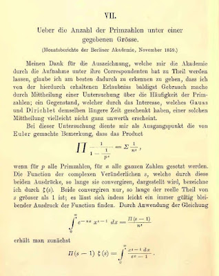
In just 10 pages he set out new ideas that have inspired generations of mathematicians even to this day. It's hard to overestimate the historic importance of his paper.
One of the new ideas Riemann introduced was the connection between the prime counting function $\pi(x)$ that we've been talking about, and a function we now call the Riemann Zeta function $\zeta(s)$. He discovered that the distribution of primes is related to the zeros of this zeta function. In fact he suggested that the zeros only occur when complex $s$ has real part $\frac{1}{2}$ and no-where else (except for trivial zeros at negative even numbers, -2, -4. -6, etc).
In concise maths, Riemann suggested:
$$ \zeta(s) = 0 \iff s = \frac{1}{2} + it$$
Sadly, he didn't prove it in his paper. And nobody has been able to prove that innocent looking statement since.
In fact this problem, the Riemann Hypothesis, is considered one of the most important mathematical unsolved problems today. It is one of the Clay Institute millennium challenges and a successful proof will attract a $1 million dollar prize.
We've talked about this important Riemann Zeta function but we haven't explained what it actually is. We'll do that next in a little more detail.
Around 1848-50, Pafnuty Chebyshev tried to prove the Prime Number Theorem. He made great progress, and proved a slightly weaker version. The theorem was finally proved in 1896, independently by both Jacques Hadamard and Charles Jean de la Vallée Poussin.
All of these great mathematicians used ideas from a chap called Bernhard Riemann who wrote a short but historic paper titled, "On the Number of Primes Less Than A Given Magnitude".
In just 10 pages he set out new ideas that have inspired generations of mathematicians even to this day. It's hard to overestimate the historic importance of his paper.
One of the new ideas Riemann introduced was the connection between the prime counting function $\pi(x)$ that we've been talking about, and a function we now call the Riemann Zeta function $\zeta(s)$. He discovered that the distribution of primes is related to the zeros of this zeta function. In fact he suggested that the zeros only occur when complex $s$ has real part $\frac{1}{2}$ and no-where else (except for trivial zeros at negative even numbers, -2, -4. -6, etc).
In concise maths, Riemann suggested:
$$ \zeta(s) = 0 \iff s = \frac{1}{2} + it$$
Sadly, he didn't prove it in his paper. And nobody has been able to prove that innocent looking statement since.
In fact this problem, the Riemann Hypothesis, is considered one of the most important mathematical unsolved problems today. It is one of the Clay Institute millennium challenges and a successful proof will attract a $1 million dollar prize.
We've talked about this important Riemann Zeta function but we haven't explained what it actually is. We'll do that next in a little more detail.
Riemann's Zeta Function
Before we dive into the Riemann Zeta function let's go back to basics and see how it came about.
Euler, one of the greatest mathematicians of all time, was interested in infinite series, that is, series that go on forever.
Here's a simple example:
$$ \sum_{n=1}^{\infty} {n} = 1 + 2 + 3 + 4 + \cdots $$
As we keep adding these ever increasing numbers, the sum gets larger and larger and larger. Loosely speaking, the sum of this series is infinity.
What about this one?
$$ \sum_{n=1}^{\infty} {\frac{1}{2n}} = \frac{1}{1} + \frac{1}{2} + \frac{1}{4} + \frac{1}{8} + \cdots $$
We can see that numbers in this series get smaller and smaller and smaller. Adding these numbers, we can see that the sum gets closer and closer to 2. We can imagine that if we did somehow add the whole infinite series, the sum would be 2. Some people don't like that leap, and prefer to say that in the limit, as $n$ goes to infinity, the sum goes to 2. That's a perfectly fine way to think about it.
Let's look at another one:
$$ \sum_{n=1}^{\infty} {\frac{1}{n}} = \frac{1}{1} + \frac{1}{2} + \frac{1}{3} + \frac{1}{4} + \cdots $$
Looking at this series, we can see the numbers get smaller and smaller. In fact, each number is half the previous number. Does that mean the sum of the infinite series is some finite number? It may surprise you that the answer is no. This series, called the harmonic series, does actually grow to infinity, but does so very slowly.
The lesson from that last harmonic series is that it isn't always obvious whether an infinite series converges to a finite value, or whether it diverges to infinity.
Anyway, Euler was interested in series of this form:
$$ \zeta(s) = \sum_{n=1}^{\infty} {\frac{1}{n^s}} = \frac{1}{1^s} + \frac{1}{2^s} + \frac{1}{3^s} + \frac{1}{4^s} + \cdots $$
We can see there's a new variable $s$ which could be any number, like $s=4$ or $s=100$. For $s=2$ this series is
$$
\begin{align}
\zeta(2) = \sum_{n=1}^{\infty} {\frac{1}{n^2}} & = \frac{1}{1^2} + \frac{1}{2^2} + \frac{1}{3^2} + \frac{1}{4^2} + \cdots \\
& = 1+ \frac{1}{4} + \frac{1}{9} + \frac{1}{16} + \cdots \\
\end{align}
$$
Different values of $s$ give different series. The general form $\zeta(s)$ is called a zeta function.
It's natural to ask whether the series created by different values of $s$ converge. Maybe they all do? Maybe none do? Maybe some of them do and some don't.
Let's see what happens when $s=1$. The series becomes $\zeta(1) = \frac{1}{1} + \frac{1}{2} + \frac{1}{3} + \frac{1}{4} + \cdots$ which is the harmonic series we saw earlier, and we know this doesn't converge.
What about $s=2$. The series becomes $\zeta(2) = \frac{1}{1} + \frac{1}{4} + \frac{1}{9} + \frac{1}{16} + \cdots$. It turns out that this series does converge, and actually converges to $\frac{\pi^2}{6}$.
Is there a way to see which values of $s$ create series that do converge? The usual simple ratio test to see if a series converges is inconclusive.
Let's get creative! Have a look at the following picture:

We can see that the area of the rectangles is always less than the area under the curve. If the rectangles have width 1 and height $\frac{1}{n^s}$, that means:
$$ \sum_{n=1}^{\infty}\frac{1}{n^s} < 1 + \int_{1}^{\infty} \frac{1}{t^s} \, dt $$
Doing that integral is easy - just as we learned at school:
$$
\begin{align}
\int_{1}^{\infty} \frac{1}{t^s} \, dt & = \lim_{a \to \infty} \int_{1}^{a} \frac{1}{t^s} \, dt \\
& = \lim_{a \to \infty} \left[\frac{1}{1-s}t^{1-s}\right]_1^{a} \\
& = \lim_{a \to \infty} \frac{1}{1-s}a^{1-s}-\frac{1}{1-s} \\
\end{align}
$$
Now, we can see that as $a$ gets larger and larger towards $\infty$, the only way that expression is going to converge is if that $a^{1-s}$ doesn't grow larger and larger. That means $a$ must be raised to a negative number. That is, $1-s < 0$, or $s > 1$.
So, to summarise, if $ \zeta(s) = \sum_{n=1}^{\infty}\frac{1}{n^s} $ is always less than $ 1 + \int_{1}^{\infty} \frac{1}{t^s} \, dt $, which only converges if $s > 1$ .. we have our condition that the zeta function only converges if $s > 1$. Phew!
You can read more about this technique here [link], and I received help here [link].
Now that we know the $\zeta(s)$ function only works when $s > 1$, let's plot it.

The code to do this is really simple. We simply create an evenly spaced list of numbers, from 1.1 to 9.9, spaced every 0.1. We then calculate $\zeta(s)$ for all these values of $s$, and plot a graph. We could have hand-coded our own function to work out $\zeta(s)$ by summing, say the first 10 or 100 terms in the series, but we can use the convenience function provided by the popular mpmath library.
A python notebook showing the code is here:
We can see that for large $s$ the value of $\zeta(s)$ gets smaller and smaller towards 1. That makes sense, because the fractions in the series get smaller and smaller. We can also see that as $s$ gets closer to 1, the value of $\zeta(s)$ gets bigger and bigger.
Overall, we have to admit the visualisation isn't that interesting.
Into the Complex Plane
Riemann took Euler's zeta function and explored what it looked like when the parameter $s$ is not just a whole number, or even a real number, but a complex number.We have to ask ourselves, could this work? Does the series converge, and if so, where does does it converge and where doesn't it converge?
Previously we used an integral test to find for which real values of $s$ the zeta function converged. We arrived at an expression:
$$ \lim_{a \to \infty} a^{1-s} $$
which only converges if $s > 1$. Does this still work when s is complex? Let's set $s = x + iy$,
$$
\begin{align}
a^{1-s} & = a^{1-x-iy} \\
& = a^{1-x}a^{-iy}
\end{align}
$$
That first bit $a^{1-x}$ converges when $x>1$ which is saying that the real part of $s$ must be more than 1. That's good, it's compatible with our previous conclusion. We'd be in trouble if it wasn't!
The second bit $a^{-iy}$ can be rewritten as $e^{-iy\ln{a}}$ which has a magnitude of 1, and so doesn't effect convergence. Remember that $e^{i\theta} = \cos(\theta) + i\sin(\theta)$ which are the coordinates of a unit circle on the complex plane. As $a$ grows larger and larger, $a^{-iy}$ just orbits around a circle of radius 1.
So, the zeta function $\zeta(s)$ works when s is complex, as long as the real part of $s$ is more than 1.
This should be more interesting to visualise as the complex plane is two dimensional. The following shows a plot of the complex plane with real range 1.01 to 6.01 and imaginary range -2.5i to 2.5i. The colours represent the absolute value of $\zeta(s)$.

Of course, if we only look at the absolute value of the complex values of the feta function, we're losing information on the real and imaginary parts. So let's rerun the plot but this time base the colours on the real part of $\zeta(s)$.

And again, but with the imaginary part.

The code for creating this is plot is in a python notebook:
Looking at these plots, we can see there's a lot going on around the the point (1+0i). The plot of absolute values shows that $|\zeta(s)|$ grows large at this point. We can imagine a kind of stalagmite at this point! Interestingly the plot of the real part of the zeta function shows the action shifted right a little, and the plot of the imaginary part shows action between the point (1+0i) continuing to the right. worth coming back to this to explore it further.
Is that the only point of interest? Let's zoom out to a wider viewpoint with real part ranging from 1.01 to 31.01 and imaginary part -15i to +15i. The following shows all three absolute, real and imaginary part plots.

This wider view shows us that there is interesting stuff happening at points other than (1+0i). It looks like there might be something happening to the left of (1+14i) and (1-14i) ... but how can this be? Surely, the zeta function only exists on the complex plane where the real part if greater than 1. Hmmmm....
Let's make a contour plot to give us a different insight into the function. The lines of a contour plot try to follow similar values. The Python matplotlib has a convenient contours plot function.
Click on the following to take a closer look.

The viewport is larger with real part going from 1.01 to 41.01, and the imaginary part from -20i to +20i. The contour plots not only reveal more curious action along the left hand edge, they also give a clearer view of how the zeta function behaves near that edge.
The code for creating these contour plots is in the following python notebook:
It's instructive to combine the three kinds of plot (absolute value, real and imaginary parts) so we can see them together:

Let's now return to that question we asked earlier. Those contour lines seem to point to something that's happening off the left-hand edge, $\Re(s) = 1$. It's as if the pattern was brutally cut off before we could see it in its entirety.
Let's imagine what would happen if we continued those lines.

This is really interesting. The maths tells us that the contour lines must stop at $\Re(s) = 1$ because the zeta function doesn't converge for $s \le 1$. We can't argue with the maths. And yet, the picture suggests very strongly that the pattern does continue.
Curiouser and curiouser!
Analytic Continuation
One of several strokes of genius that Riemann had was to resolve that puzzle above.
Have a look at the following infinite series:
$$ f(x) = 1 + x + x^2 + x^3 + x^4 + x^5 + ... $$
Have a look at the following infinite series:
$$ f(x) = 1 + x + x^2 + x^3 + x^4 + x^5 + ... $$
We already know that this series only converges if each successive term doesn't increase, that is $x < 1$. What if we used a complex number $z$ instead of a plain normal number $x$?
$$ f(z) = 1 + z + z^2 + z^3 + z^4 + z^5 + ... $$
How do we decide for which $z$ this converges? If we write $z$ in the polar coordinate form $z = r \cdot e^{i\theta}$, we can see that
$$ f(z) = 1 + r \cdot e^{i\theta} + r^2 \cdot e^{i2\theta} + r ^3 \cdot e^{i3\theta} + ... $$
The ratio test gives us
$$
\begin{align}
\lim_{n \to \infty} \vert \frac { r ^{n+1} \cdot e^{i(n+1)\theta}} { r^n \cdot e^{in\theta}} \vert & < 1 \\
\\
\lim_{n \to \infty} \vert r \cdot e^{i\theta} \vert & < 1 \\
\\
\vert r \vert & < 1 \\
\end{align}
$$
So the series converges as long as the complex number $z$ is within the unit circle, as shown in the next picture.

Now, let's take a different perspective on that series.
$$
\begin{align}
f(z) & = 1 + z + z^2 + z^3 + z^4 + z^5 + ... \\
z \cdot (f(z) & = z + z^2 + z^3 + z^4 + z^5 + z^6 + ... \\
1 + z \cdot (f(z) & = 1 + z + z^2 + z^3 + z^4 + z^5 + ... \\
& = f(z) \\
1 &= (1-z) \cdot f(z) \\
f(z) &= \frac{1}{1 - z} \\
\end{align}
$$
So we have a simple expression for the sum of that series. But this expression doesn't itself suggest that $\vert z \vert < 1$. It only suggests that $z \ne 1$.
What's going on ?!
One way to think about this is that $f(z) = \frac{1}{1 - z}$ is function which works over the entire complex plane, except at $z = 1$, and that the series $f(z) = 1 + z + z^2 + z^3 + z^4 + z^5 + ... $ is just a representation which works only for $\vert z \vert < 1$. In fact, it is just one of many representations. Another, slightly more complicated, representation is $f(z) = \int_0^{\infty} {e^{-t(1-z}}\,dt$ which works over $\Re(z) < 1$, which also covers the left-half plane.
What analytic continuation does is to take a representation which has a limited domain over which it works, and tries to find a different representation which works over a different domain. If we're lucky we might find the function that works everywhere, or at least the maximum possible.
There are several methods to do this analytic continuation, and they all depend on the fact that if two representations overlap, and have the same values there, then they are compatible in quite a strong sense. Actually doing the continuation is fairly heavy with algebra so we won't do it here. What we can do is get an intuitive feel for how and why analytic continuation works.
Have a look at the following, which shows the same zone of convergence of the series representation as before.

This time we're noting that the series is in fact the Taylor expansion of $f(z) = \frac{1}{1 - z}$ about $z=0$ and the radius of converge is the distance from $z=0$ to the nearest pole, which is at $z=1$ in this example. A pole is just a point where the function isn't defined and in the limit approaches infinity. Think of pole holding up a tent cloth!
Now, what happens if we take a Taylor series expansion of the same $f(z) = \frac{1}{1 - z}$ but about a different point, $z = 1 + 0.5i$, or example.

The resultant series, which is fairly easy to work out, has a radius of convergence centred about $z = 1 + 0.5i$ and extends to the pole. In fact that circle is smaller than our previous one because the pole is closer. But notice that this new domain covers a part of the complex plane that the previous circle didn't.
We've extended the domain! And we can keep doing it ..

We can keep doing this until we cover the entire complex plane, but excluding that pole of course. This technique is especially useful if we didn't know the true function, but only series representations which have limited domains.
Can this be done with the Riemann Zeta function, which in the series form, only works for $\Re(z) > 1$. Those contour plots strongly suggested it could be. The answer is yes! In fact it can be extended to the entire complex plane, and that continuation has only one pole at $z=1$ and many zeros. We won't do it here because the algebra is heavy.
What we can do is use software like the Python mpmath library to visualise the rest of the Riemann Zeta function.

We can see the values do continue naturally from that hard boundary we have before at $\re(z) = 1$. We can also see that the values are a lot more varying in the left half of the complex plane. To the right the function seems to be very calm, boring even.
Interestingly, we can see what look like zeros of the zeta function going up the line $\Re(z) = \frac{1}{2}$. That's worth a closer look.
Let's see what a contour plots can show us.

Those zeros have become really clear. There are three things to note:
- There are zeros up the line $\Re(z) = \frac{1}{2}$
- There are zeros at every negative even number on the real line, -2, -4, -6, -8, ...
- There is one pole at 1.
For completeness, the following plots compare the real and imaginary contours. The values, which cover a very broad range, have been subjected to a natural log just to aid visualisation.

The code for these plots are online:
- colour plots: https://drive.google.com/open?id=13CLcA8at9JoHQJw7lo0sPNucCcAabtJ2
- contour plots: https://drive.google.com/open?id=18jgeJg_8fa1ka4AxoC5Ek-AKdz7ZxW0i
The following is a higher resolution plot combining the colour plot and the contours for absolute and real parts.

Zeta Zeros - $1 Million Prize!
Mathematicians have proved:- there is only one pole in the version of the Riemann Zeta function extended to the entire complex plane
- there are zeros at $-2n$, the negative odd real numbers
But, mathematicians have not yet proved that the other, so-called non-trivial zeros, are all on the vertical line $\Re(z) = \frac{1}{2}$.
If you can do that, or disprove it, you'll be awarded 1 million dollars.
In 1903, 15 non-trivial zeros of the Riemann Zeta function were found. By 2004, $10^{13}$ zeros were found, all on the line $\Re(z) = \frac{1}{2}$. That looks like extremely convincing evidence - but it is still not proof.
This challenge has been open since Riemann's 1859 paper, and was part of Hilbert's 1900 collection of unsolved important problems, as well as the Clay Institute's millennial problems set out in the year 2000.
More Reading
- Nice easy-going video on visualising the Riemann Zeta function https://www.youtube.com/watch?v=sD0NjbwqlYw
- Barry Mazur "A Lecture on Primes and the Riemann Hypothesis" (video) https://www.youtube.com/watch?v=way0jAWpjZA
- One of the best explanations of the Riemann Hypothesis: https://medium.com/@JorgenVeisdal/the-riemann-hypothesis-explained-fa01c1f75d3f
- The official Clay Institute millennium challenge: http://www.claymath.org/millennium-problems/riemann-hypothesis
- English translation of Riemann's "One The Number of Primes Less Than A Given Magnitude": http://www.claymath.org/sites/default/files/ezeta.pdf
- A good overview of the Prime Number Theorem and the Riemann Hypothesis: https://thatsmaths.com/2014/02/27/the-prime-number-theorem/
- A very readable introduction to analytic continuation: http://www.mathpages.com/home/kmath649/kmath649.htm
- Another intro to analytic continuation showing other methods: https://www.colorado.edu/amath/sites/default/files/attached-files/pade_analytic_continuation.pdf
- Download the zeros of the Riemann Zeta function: http://www.dtc.umn.edu/~odlyzko/zeta_tables/