
Previously:
- Part 1 introduced the idea of adversarial learning and we started to build the machinery of a GAN implementation.
- Part 2 we extended our code to learn a simple 1-dimensional pattern 1010.
In this post we'll develop our GAN further to to learn, not a single pattern, but a collection of patterns. We'll also start to see some of the difficulties of training a GAN, which we'll try to address in the next post.
In this post I won't focus too much in PyTorch as that will distract us from exploring the ideas. The PyTorch code is essentially the same as what we developed previously, with the only differences being relatively boring details like how to load the training data and display 2-dimensional images. All the code will be provided on github for you to examine.
MNIST Dataset of Handwritten Digits
The patterns our GAN will be learning to generate are hand written digits 0-9. There is a very well known and used dataset called MNIST. It contains 60,000 images intended for training and 10,000 intended for testing. The images are 28x28 pixels in size, and are provided with the correct labels.
You can read more about how to get and understand the dataset here: link.
Big Picture
Before we dive into coding let's draw a big picture view of our GAN architecture.

There are one key difference from our previous GAN. The training data is no longer a single 1-dimensional pattern 1010, but is a collection of 2-dimensional images. Each image in the training dataset is different to any other one.
The other differences are just extensions from 1-dimensional data to 2-dimensional data. For example, the output of the generator is a 28x28 image, just like the training data. The discriminator now accepts a 2-dimensional 28x28 image, but still outputs 1 for real and 0 for fake.
With the overview in our minds, let's work through each section, step by step.
Discriminator
The job of the discriminator is to successfully distinguish between images from the real training data set, and images coming from the generator.The question for us is what architecture, size and shape should the discriminator have? Should it have many layers? Should it use convolutions or the traditional fully connected nodes? What activation function should we use? How big should the layers be?
There isn't a perfect answer to this question. In fact, deciding exactly what network architecture is suitable for a task is an open research question.
A good approach for us is to start with a small simple neural network and check that it can first learn to classify the MNIST dataset. If a smaller network works for us, then we don't want a larger one that will be harder to train, require more computational resource and risks behaving in unexpected and unwanted ways.
The loose rationale is that if our small network can learn to classify MNIST data against the 10 labels, then it should have enough capacity to perform the simpler task of classifying against 2 labels real/false.
Let's start with very simple classifying network:
- Input layer of 784 nodes to match the 32x32 image pixels.
- Hidden middle layer of 200 nodes, with a simple sigmoid activation.
- Output layer of 10 nodes, one for each class 0-9, with a simple sigmoid activation to match the desired 0-1 output range.
- Binary cross entropy loss (BCELoss) as it penalises incorrect classifications stronger than the vanilla mean squared error loss (MSELoss).
- Simple stochastic gradient descent (SGD) rather than anything fancy like Adam.
The code that implements this simple architecture is:
# define neural network layers
self.model = nn.Sequential(
    nn.Linear(784, 200),
    nn.Sigmoid(),
    nn.Linear(200, 10),
    nn.Sigmoid()
)

# create error function
self.error_function = torch.nn.BCELoss()

# create optimiser, using simple stochastic gradient descent
self.optimiser = torch.optim.SGD(self.parameters(), lr=0.01)
Training this classifier on the 60,000 training images and testing it on the 10,000 test images gives a very respectable 90% accuracy. Not bad for a very simple network.
The following shows the classifier loss as training progresses for 3 epochs.

And the following shows a manual check to see if an image is correctly classified. We can see the confidence in the label 2 is high.

You can see the full code for this MNIST classifier online:
This confirms this simple network can learn to classify MNIST so we can reasonably assume it has the capacity to learn the simpler task of discriminating between real and generated images.
The discriminator network only has one output so the last layer is changed to have just 1 output node.
# define neural network layers
self.model = nn.Sequential(
    nn.Linear(784, 200),
    nn.Sigmoid(),
    nn.Linear(200, 1),
    nn.Sigmoid()
)
Couldn't be much simpler!
Is there any way can gain some confidence this discriminator can work with a single node output, beyond the reasonable argument we just made? Yes - we can train it to output 1 when seeing real images, and output 0 when seeing random noise.
The following shows the discriminator loss getting smaller when trained on real images and random noise. While we're developing the code, we'll use the smaller 10,000 training set rather than the larger 60,000 training set.

Let's manually test the discriminator with real image and random inputs.
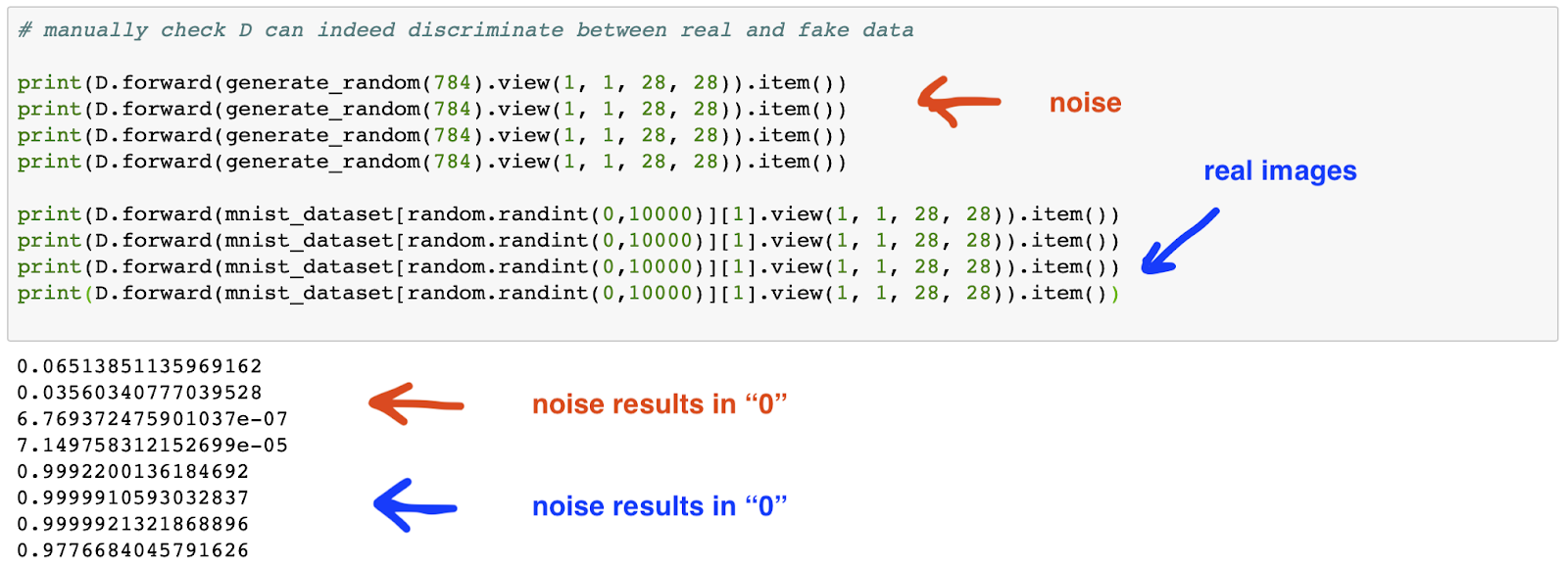
The discriminator seems to be capable of learning the difference between real images and noise, which although not an ideal test of its capability, provides some confidence that we can include it in the GAN.
Generator
The generator needs to take random noise as input and output a 28x28 image. There are two questions that we need to answer:- what size of random noise array should we use?
- what kind of neural network do we need between the input and output layers?
On the first question, there isn't an analytic answer we'll have to use an educated guess. Too small an input and we make it hard for the generator to provide a diverse set of output images. Too large and we waste computational resource, making the network hard to train. Given the output image has 28*28 = 784 a good starting guess is 100.
On the second question we should follow our previous approach of starting as small as possible and only growing the size and complexity if needed. If we only had one hidden layer, what size should it be? If the output is 784 nodes, this hidden layer needs to provide the network with the capacity to learn different images. This suggests a size of larger than 784, but let's see if we can get a smaller 500 to work.
So let's start with a generator network with the following:
- Input layer of 100 nodes to receive the random noise.
- Hidden middle layer of 500 nodes, with a simple sigmoid activation.
- Output layer of 784 nodes to form 28x28 images, with a simple sigmoid to match the target 0-1 range.
- The same simple BCE loss and SGD gradient descent methods as the discriminator.
The following code is is the model for generator:
# define neural network layers
self.model = nn.Sequential(
    View((1,100)),

    nn.Linear(100, 500),
    nn.Sigmoid(),

    nn.Linear(500, 784),
    nn.Sigmoid(),

    View((1,1,28,28))
)
Again, very simple.
Let's remind ourselves of the training process. The following steps are repeated for all the training images:
- train the discriminator on a real image with a target output of 1.0 (true)
- train the discriminator on a generated image with a target output of 0.0 (false)
- train the generator to cause the discriminator to produce a 1.0 (true)
The training code looks like this:
# train Discriminator and Generator

epochs = 1

for i in range(epochs):
    print('training epoch', i+1, "of", epochs)

    for label, image_data_tensor, target_tensor in mnist_dataset:

        # train discriminator on real data
        D.train(image_data_tensor.view(1, 1, 28, 28), torch.FloatTensor([1.0]).view(1,1))

        # train discriminator on false
        # use detach() so only D is updated, not G
        D.train(G.forward(generate_random(100).view(1, 1, 10, 10)).detach(), torch.FloatTensor([0.0]).view(1,1))

        # train generator
        G.train(D, generate_random(100).view(1, 1, 10, 10), torch.FloatTensor([1.0]).view(1,1))

        pass

    pass
You can see an outer loop which allows the training to be repeated for a given number of epochs.
Using the smaller 10,000 training set, the discriminator loss looks like this:

The loss fall quickly as the discriminator learns to tell real and generated images apart. Remember, in the early stages, the generator will not be creating good images, and the discriminator will find it easy to tell them apart from the real images. As training continues the generator gets better, the discriminator seems to get worse again, but towards the end approaches a loss of 0.5 which is the theoretical equilibrium when it can't tell real and generated images apart.
The generator loss - or more accurately the discriminator loss caused generated images - rises as training progresses because it gets better at fooling the discriminator.

Let's see a sample of six generated images after one round of training - 1 epoch.

There's good news and bad. The good news is that the images are not random noise and have some kind of structure in the middle of the area. The bad news is that the structures aren't recognisable as digits.
Let's run another round of training.

We can see the discriminator loss falls below 0.5 and the generator loss rises. The resulting images are all similar and very spiky (high contrast). What appears to have happened is that the generator has found a solution that is very good at fooling the discriminator.
Let's try four more rounds of training so we have a total of 6 epochs.

That hasn't improved the results. The generator is producing even more spiky images. The high contrast which means it has high confidence that they will fool the discriminator.
The two problems we have are:
- the generator creates the same/similar images from different random inputs
- the images don't look like digits
The problem of a generator learning only one pattern, albeit a pattern that does fool the discriminator. The problem of the generator overwhelming the discriminator so the loss isn't balanced around 0.5 is because we've not reached an equilibrium between the adversarial discriminator and generator.
The code for this initial attempt at an image generating GAN is online:
GANS Are Hard To Train
We've just seen how GAN training can partially fail. The generator and discriminator were learning, but the state they ended up in wasn't what we wanted. We wanted the generator to be able to produce a range of images that look like digits.Compared to normal neural network architectures, GANs are still a relatively new idea and the methods for training them are aren't yet fully understood. It is an active area of research.
It is possible for GAN training to totally fail with no convergence happening at all. We were lucky our simple network didn't see that.
If we can get our GANs to converge, the main issue is the generator not producing a range of images, like we saw earlier. Have a look at the following diagram from this paper (pdf).

The diagram shows real data which can be one of 8 different types. For example, we might have images of digits that are just 0-7. The diagram also shows a trained generator only producing images that match one of the 8 types. This is called mode collapse - the generator has found one solution that works and has fallen into it, and is unable to find other solutions that also work.
So how do we fix this?
Most of the current advice for turning GANs is heuristic or based on educate guesses. You'll find some of the suggestions apparently based on theory contradict each other. Some of the improvements suggested are architectural - even using several generators, instead of one.
There can be several causes of mode collapse, or even non-convergence. Here are some:
- a mismatch between the discriminator and generator - the adversarial game only works if both improve and one doesn't leave the other behind
- unbalanced training data (the MNIST training data is balanced)
- learning algorithms that suffer saturation or diminished gradients just like normal neural networks
Let's see if we can make small adjustments that fix this mode collapse.
Improving Training Updates
One of the most common changes made to GAN neural networks is the method by which the errors are used to update the network weights.The basic stochastic gradient descent (SGD) is fine in many cases. It is also simple and fast, both of which are merits. One of its disadvantages is that it can jump about the error minimum that it is trying to get to as it isn't the best at adapting its weight change steps.
There are more sophisticated methods like the very popular Adam (adaptive momentum estimation) which has two key features:
- it has individual learning rates for each parameter, not one general learning rate
- the individual learning rates are adapted based on recent changes (momentum)
A very good explanation of Adam is here:
The code change to use Adam is very simple. Note with Adam we typically use much smaller learning rates compared to SGD.
# create optimiser, using simple stochastic gradient descent
self.optimiser = torch.optim.Adam(self.parameters(), lr=0.0001)
A second improvement is within the neural networks themselves. The logistic activation function is simple and was historically popular. However, one of its major weaknesses is vanishing gradients for much if its input range. You can see this in the following graph. Gradients are needed for the update process, and if the network becomes saturated, or just has large values passing through it, then diminished gradients severely limit learning.

A very good answer is to use the rectified linear unit ReLU, or an improved version of it called a LeakyReLU.

The gradient on the right hand side remains strong. The small gradient on the left avoid the zero gradient problem leading to "dead ReLUs".
One more change that is also very common is to add normalisation layers into the network. A simple variant, called LayerNorm in PyTorch, is to take all the signals out of a network layer and normalise them so they they are centred about 0 and have a standard deviation of 1.
The following shows the updated discriminator:
# create optimiser, using simple stochastic gradient descent
# define neural network layers
self.model = nn.Sequential(
    ((1, 784)),
    nn.Linear(784, 200),
    nn.LeakyReLU(),

    nn.LayerNorm(200),

    nn.Linear(200, 1),
    nn.Sigmoid()
)
And the following is the updated generator:
# define neural network layers
self.model = nn.Sequential(
    View((1,100)),

    nn.Linear(100, 500),
    nn.LeakyReLU(0.2),

    nn.LayerNorm(500),

    nn.Linear(500, 784),
    nn.Sigmoid(),

    View((1,1,28,28))
)
Let's see if these improvements actually result in better generated images.
Here are the results from one round of training on the smaller 10,000 test set.

We can see the images from the generator now starting to look like real numbers. There are some that look like a 3 and some that could be a 9, or the beginnings of a 7 or a 1.
The discriminator loss follows a different pattern. The loss falls very rapidly due to the improvements we've made. However after a while, the losses start to increase as the generator starts to learns how to fool it. If you look closely, the losses in the discriminator caused by the generator are large.
Let's run the training again for a second epoch.

The digits are improving. The discriminator loss is still mostly low but with more samples being pulled upwards. We can see how over time the average might approach the theoretical 0.5.
Let's see what 4 epochs does:

This is a mixed picture. We have some digits much better defined like the 5 and 3, but some that are degrading.
And here's the result of 8 epochs.

Some, but not all, of the generated images are starting to look really good now.
The following is the result of 2 epochs training on the bigger 60,000 MNIST training set.

That's a much better result. The benefit is not just from the larger number of training examples, but the fact that they are different. Multiple epochs on a smaller dataset means repeating the same, and so less diverse, set of images.
You can explore the GAN code which includes these improvements here:
Discussion
We've succeeded in training our generator to create images that look very like hand-written digits. And we did this while keeping our GAN neural networks very simple. We didn't need to have lots of layers or have more complex schemes like convolution layers.We did experience the mode-collapse issue and overcame it with a stronger Adam optimiser, using the ReLU activation and the layer normalisation to help stabilise learning.
It is easy to understand how these improvements improve GAN convergence, but it is not immediately clear how these improvements, which apply to both the generator and discriminator, help avoid mode collapse.
The following chart shows the results of using combinations of Adam, layer normalisation and the ReLU activation, using 4 epochs of training on the smaller 10,000 MNIST test set.

Although not rigorous, these initial experiments suggest that the best results are from all three optimisations applied together. Individually, Adam on its own has the least benefit and seems not to break the mode collapse. LeakyReLU and layer normalisation break mode collapse. It's not overly clear but I think LeakyReLU has the most benefit.
In the next Part 4 of this series we'll try to learn more photo-realistic colour images, where we might have to expand our networks to use convolution and de-convolutions to learn localised image features.
More Reading
- Excellent overview of gradient descent methods: http://ruder.io/optimizing-gradient-descent/
- A short accessible video on GANs: https://www.youtube.com/watch?v=hQv8FNaJHEA
- In-depth tutorial by Ian Goodfellow: https://arxiv.org/abs/1701.00160