Generative Adversarial Networks - Part II

This is the second in a short series of posts introducing and building generative adversarial networks, known as GANs.

In Part I we looked at the interesting architecture of adversarial learning with two learning models pitted against each other. We also built a very simple example of two nodes with adjustable parameters to get started with coding this adversarial architecture and visualising the learning as it progresses.

That example was so simple that the algebra collapsed to make the generator independent of the discriminator, but the exercise was still useful to develop the code and visualisation and avoid the additional complexity of neural networks.

We now progress to using neural networks as the learning models, but still keep both the learning task  and the neural networks as simple as possible.

PyTorch

I firmly believe in learning how to build things from scratch if we really want to understand them. We've previously learned to make our own neural networks from scratch using Python. You can read more on the blog that follows that journey.

Once we've done that it can make sense to use frameworks that make building and using neural networks easier. There are two leading choices - PyTorch and TensorFlow. Both allow easy use of GPU acceleration. Although TensforFlow is open source, its development is firmly led by Google. PyTorch has some advantages:

• it is much more open source in its development and community involvement
• it is much more pythonic, meaning code is easy to read and learn, and also to debug
• the computation graphs are dynamic allowing more interesting tasks to be done more simply

We'll be using PyTorch.

I previously wrote an intro to PyTorch. Although PyTorch itself has changed a little the explanation of its ability to automatically calculate error gradients for back propagation is still valid:

• http://makeyourownneuralnetwork.blogspot.com/2017/05/learning-mnist-with-gpu-acceleration.html

Task Overview -  Learn To Imitate 1010 Patterns

The following diagram shows an overview of our task. The architecture is the same as we saw last time - the discriminator is being trained to classify data from the training data as real, and data from the generator as fake.

This time the generator and discriminator are simple neural networks. Because neural networks need an input, the generator is fed data, which we'll discuss below.

The diagram also shows where learning happens. The discriminator learns as a result of the error in its output. Back-propagation of this error is used to calculate the weight changes in the discriminator neural network.  The generator also learns from the classification error with the neural network weight changes back-propagated all the way back to itself via the discriminator.

Training Data

The training data are patterns of four numbers of the form 1010. What we'll do is make this a little fuzzy by generating four random numbers where the first and third are close to 1, and the second and fourth are are close to 0. That means the training data could be something like [0.99, 0.01, 0.98, 0.02].

We can write a very simple function to create this fuzzy 1010 pattern:

# function to generate real data

def generate_real():
    t = torch.FloatTensor([random.uniform(0.8, 1.0),
                           random.uniform(0.0, 0.2),
                           random.uniform(0.8, 1.0),
                           random.uniform(0.0, 0.2)]).view(1, 4)
    return t

You can see we're not just returning a simple python list but turning it a PyTorch tensor which is like a numpy array, but with additional machinery needed to enable machine learning.

Feeding The Generator

The generator also creates data in the form of four numbers. If the training goes well, it will have learned to imitate the training data and create numbers that might be like [0.99, 0.02, 0.99, 0.01]. Unlike last time, this generator is a neural network and so needs an input to turn into an output. The most neutral input is four uniformly random numbers.

Again, the code for generating uniformly random numbers is very simple:

# function to generate uniform random data

def generate_random():
    t = torch.FloatTensor([random.uniform(0.0, 1.0),
                           random.uniform(0.0, 1.0),
                           random.uniform(0.0, 1.0),
                           random.uniform(0.0, 1.0)]).view(1, 4)
    return t

We can test these functions to be sure they do create data that looks right:

We can see the generate_real() function does indeed create number that are high-low-high-low.

The Discriminator

We'll use PyTorch to build the discriminator as a simple neural network. It'll need 4 input nodes because the training data examples are 4 numbers (1010). Because the discriminator is a classifier, it only needs 1 output, which can have a value of 1 for "true" and 0 for "false". To keep things simple, we'll have just one hidden layer, and it can have 3 hidden nodes. I'm pretty sure an even smaller hidden layer would work, but that experimentation is a distraction from our task here.

Neural networks are typically built by subclassing from PyTorch. We describe the size and other design elements in the __init__() constructor. We also need to describe how the inputs work their way to become outputs, via network layers and activation functions. By convention this is described in a method called forward().

The following shows the code for a discriminator class:

## discriminator class

class Discriminator(nn.Module):
    
    def __init__(self):
        # initialise parent pytorch class
        super().__init__()
        
        # define the layers and their sizes, turn off bias
        self.linear_ih = nn.Linear(4, 3, bias=False)
        self.linear_ho = nn.Linear(3, 1, bias=False)
        
        # define activation function
        self.activation = nn.Sigmoid()
        
        # create error function
        self.error_function = torch.nn.MSELoss()

        # create optimiser, using simple stochastic gradient descent
        self.optimiser = torch.optim.SGD(self.parameters(), lr=0.01)
        
        # accumulator for progress
        self.progress = []
        pass
    
    
    def forward(self, inputs):        
        # combine input layer signals into hidden layer
        hidden_inputs = self.linear_ih(inputs)
        # apply sigmiod activation function
        hidden_outputs = self.activation(hidden_inputs)
        
        # combine hidden layer signals into output layer
        final_inputs = self.linear_ho(hidden_outputs)
        # apply sigmiod activation function
        final_outputs = self.activation(final_inputs)
        
        return final_outputs
    
    
    def train(self, inputs, targets):
        # calculate the output of the network
        output = self.forward(inputs)
        
        # calculate error
        loss = self.error_function(output, targets)
        
        # accumulate error
        self.progress.append(loss.item())

        # zero gradients, perform a backward pass, and update the weights.
        self.optimiser.zero_grad()
        loss.backward()
        self.optimiser.step()
        pass
    
    
    def plot_progress(self):
        df = pandas.DataFrame(self.progress, columns=['loss'])
        df.plot(ylim=(0, 0.5), figsize=(16,8), alpha=0.1, marker='.', grid=True, yticks=(0, 0.25, 0.5))
        pass
    
    pass

You can see the hidden (middle) layer combines the inputs as a linear combination, and we use a simple sigmoid activation function. The same is done to take the outputs of the hidden layer to the final layer, which is just a single node. The error function is again a simple mean squared error. The optimiser, which decides how to change the neural network weights, is also a very simple stochastic gradient descent. We've deberately chosen simple options as our focus here is on getting a basic GAN up and running, not worrying about fine details.

The train() method is pretty self-explanatory too. The inputs are pushed through the network using the forward() function, and the output is compared to the target to give the error, conventionally called the loss. I've added code to append the loss to a list so that we can visualise how it changes over many training runs. The last three lines of code in the train() method are standard PyTorch - we need to zero the gradients from any previous runs, use the latest loss to back propagate and calculate new error gradients, and the change the weights.

Before we move onto the generator, let's make sure our discriminator works. The following code

    
 # test discriminator itself works

D = Discriminator()

for i in range(10000):
    D.train(generate_real(), torch.FloatTensor([1.0]))
    D.train(generate_false(), torch.FloatTensor([0.0]))
    pass

You can see we're giving the discriminator examples of fuzzy 1010 data from generate_real() and telling it the correct classification is 1.0. We're also giving the discriminator examples of false data and telling it the correct classification is 0.0. The generate_false() simply provides a fuzzy 0101 pattern.

Let's visualise the discriminator loss over these 10,000 training sessions.

That looks like the right shape. Over training sessions, the error is falling, which means the discriminator is getting better at learning the training data. You might be wondering why the values start around 0.25 and not 0.5. That's because on average each position in the sequence 1010 will be wring half the time, so the sum on average is 2, the mean is 0.5 and the square of the mean is 0.25. So "half right" will be 0.25 on the graphs, not 0.5.

The reason that plot of errors seem to have two modes at the start is because in the early stages of learning, the network will have an average accuracy for classifying real data that is distinct from the average accuracy against random data.

Let's manually test the discriminator by feeding it data we know to be true and false:

Fed a 0101 pattern, the output is a low 0.05 (false). Fed a 1010 pattern, the output is a high 0.94 (true). That confirms the discriminator is working correctly.

The Generator

Let's now build the generator. Let's remind ourselves what it is. It is a learning model that learns to get better at generating data that looks real. As we're using a using a neural network to do this learning, we need to think about its architecture. We can use 4 output nodes for the four positions of the 1010 pattern. The input and hidden layers have greater freedom, but for simplicity we'll go for 4 nodes in each of these. Any smaller and we risk limiting the expressive capacity of the network.

The generator neural network needs an input. If we think about it, the output depends on the input. If we're tuning the network to learn to give a desired output, we want the inputs to, at minimum, not make that task difficult by being biased. This points to a uniform randomness as the inputs to the network.

The code for the generator class is almost identical to the discriminator - they are both neural networks, passing signals from every node in one layer to every node in the next layer, using the same sigmoid activation function, and the same mean squared error function.

    
# generator class

class Generator(nn.Module):
    
    def __init__(self):
        # initialise parent pytorch class
        super().__init__()
        
        # define the layers and their sizes, turn off bias
        self.linear_ih = nn.Linear(4, 4, bias=False)
        self.linear_ho = nn.Linear(4, 4, bias=False)
        
        # define activation function
        self.activation = nn.Sigmoid()
        
        # create error function
        self.error_function = torch.nn.MSELoss()

        # create optimiser, using simple stochastic gradient descent
        self.optimiser = torch.optim.SGD(self.parameters(), lr=0.01)
        
        # accumulator for progress
        self.progress = []
        
        # counter and array for outputting images
        self.counter = 0;
        self.image_array_list = [];
        pass
    
    
    def forward(self, inputs):        
        # combine input layer signals into hidden layer
        hidden_inputs = self.linear_ih(inputs)
        # apply sigmiod activation function
        hidden_outputs = self.activation(hidden_inputs)
        
        # combine hidden layer signals into output layer
        final_inputs = self.linear_ho(hidden_outputs)
        # apply sigmiod activation function
        final_outputs = self.activation(final_inputs)
        
        return final_outputs
    
    
    def train(self, D, inputs, targets):
        # calculate the output of the network
        g_output = self.forward(inputs)
        
        # pass onto Discriminator
        d_output = D.forward(g_output)
        
        # calculate error
        loss = D.error_function(d_output, targets)
        
        # calculate how far wrong the generator for purposes of plotting
        # note we're using knowledge about real data here
        g_loss = self.error_function(g_output, torch.FloatTensor([0.9, 0.0, 0.9, 0.0]))
        
        # accumulate error
        self.progress.append(g_loss.item())

        # zero gradients, perform a backward pass, and update the weights.
        self.optimiser.zero_grad()
        loss.backward()
        self.optimiser.step()
        
        # increase counter and add row to image
        self.counter += 1;
        if (self.counter % 1000 == 0):
            self.image_array_list.append(g_output.detach().numpy())
            pass
        
        pass
    
    
    def plot_progress(self):
        df = pandas.DataFrame(self.progress, columns=['loss'])
        df.plot(ylim=(0, 0.5), figsize=(16,8), alpha=0.1, marker='.', grid=True, yticks=(0, 0.25, 0.5))
        pass
    
    
    def plot_images(self):
        plt.figure(figsize = (16,8))
        plt.imshow(numpy.concatenate(self.image_array_list).T, interpolation='none', cmap='Blues')
        pass
    
    pass

Although most of the generator code is similar to that of the discriminator, the training is different. Here we pass the inputs through the generator as normal to give the outputs. However, we aren't learning by comparing these outputs with real data. Remember, the generator doesn't see the real data. It only learns by looking a how well it convinced the discriminator. So we push the generator outputs through the discriminator to get a classification. We want that to be real or 1.0.

The error function, which decides how we update the network weights, compares the classifier output with what it should be, 1.0. The way PyTorch works, the act of performing calculations on PyTorch tensors, starting with the random inputs to the generator, through to the output of the discriminator, means PyTorch internally calculates the error gradients from the classification error all the way back through the discriminator weights to the generator weights.

However - we don't want to change the discriminator weights. We aren't training the discriminator to recognise the generator outputs as real. We're only training the generator. Luckily, the call to self.optimiser.step() referred only to the generator parameters, so this is easy to do and doesn't require extra coding.

We have the same extra code to keep a log of the generator errors just like before, but this time we are using knowledge of what real data should look like to make the comparison. Look at the code yourself to confirm that knowledge is not used to train the generator itself. It's only used to help us visualise progress, and can be removed at any time.

We also have additional code which takes a snapshot of the generator outputs at every 1000 training steps so we can visualise the patterns it creates.

Adversarial Training

The training of this adversarial architecture takes three distinct step, repeated many times:

• showing the discriminator a real data example, and telling it the classification should be 1.0
• showing the discriminator the output of the generator and telling it the classification should be 0.0
• showing the discriminator the output of the generator and telling the generator the result should be 1.0

The first two steps train the discriminator to get good at separating real and false data. The third step trains the generator to get create real looking data that can get past the discriminator.

The code for this three step training is simple:

    
# create Discriminator and Generator

D = Discriminator()
G = Generator()


# train Discriminator and Generator

for i in range(10000):
    
    # train discriminator on true
    D.train(generate_real(), torch.FloatTensor([1.0]))
    
    # train discriminator on false
    # use detach() so only D is updated, not G
    D.train(G.forward(generate_random()).detach(), torch.FloatTensor([0.0]))
    
    # train generator
    G.train(D, generate_random(), torch.FloatTensor([1.0]))
    
    pass

Let's see how the discriminator training progresses:

That's interesting!

Before, the error reduced towards zero as the discriminator got better and better at telling real data from fake data. Now the discriminator seems to be approaching a state where it isn't good at telling real data apart from the data from the generator, which itself is getting better and better at generating more realistic data. That's why the error is approaching an average of 0.25.

Let's see the error between the output of the generator compared to what we know real data should look like:

That confirms the generator is getting better and better at data that looks like 1010.

Great - we've trained a generator that successfully learns to create realistic data that the discriminator finds hard to tell apart from actual real training data!

Images

Let's visualise the snapshots the generator took of its output at every 1000 training steps.

The generator output starts indistinct, but over time, the out becomes distinctly 1010.

This visualisation is a forward look to Part III where we'll try to train a GAN to generate 2-dimensional images.

As a final check, let's manually run the generator to confirm the outputs do indeed look like 1010.

Yup - the outputs are very close to 1010.

Conclusion

We've succeeded in taking the basic adversarial architecture we discussed in Part I,  developing it to use neural networks as learning units, and applying it to a more interesting learning task.

We also used visualisation of the error and generator outputs to see, and better understand, the training process.

The key point here is that the generator never sees the real training data - yet it learns to create convincing imitations!

The code is available on github as a notebook:

• https://github.com/makeyourownalgorithmicart/makeyourownalgorithmicart/blob/master/blog/generative-adversarial-network/01_simple_gan.ipynb

More Reading

• Stanford's intro to PyTorch: https://cs230-stanford.github.io/pytorch-getting-started.html

Generative Adversarial Networks - Part I

This is the first of a short series of posts introducing and building generative adversarial networks, known as GANs.

Why GANs?

Artificial intelligence has seen huge advances in recent years, with notable achievements like computers being able to compete with humans at the notoriously difficult to master ancient game of go, self-driving cars, and voice recognition in your pocket.

Much of that recent progress has been enabled by the ability to train large neural networks as computing power has become cheaper. The training of neural networks with many layers as become known as deep learning, although that terms does cover other many-layered learning models too.

The key benefit of deep, or many-layered, neural networks is that they can learn which elements of the data are useful features. These features can usefully be reasoned about to make higher level decisions. For example, a face recognition system might learn features such as eyes and mouth. Previously we had to work out, or guess, what the right low-level features should be.

Neural networks are typically used to distill lots of data into smaller information, like a yes/no decision or a classification. But they can also be used to generate data - which can include images.

Even more recently, a new architecture emerged that led to spectacular results for generated images. The following faces are not real, they were created by a generative network (source).

In October 2018, the world-leading art auction house Christies sold the Portrait of Edmond Belamy for $432,500.

That portrait was not painted by a person, but created using a generative neural network.

The neural network architecture that generates these compelling results is known as a generative adversarial network, or GAN.

The name describes the unique adversarial way in which the networks learn.

Generative Adversarial Learning

Before we look at this unique adversarial way of learning, let's first look the typical approach to machine learning.

A model, often a neural network is fed training data, and the output of that model is compared to what the right output should be. The difference, the error, guides how internal parameters of that model are updated in an attempt to reduce the error.

For a neural network, the error is used to update the link weights that connect nodes in the network, using a method known as back propagation of the error.

This typical approach has been pervasive across many forms of machine learning.

Although he wasn't the first to explore the idea, Ian Goodfellow's 2014 paper (pdf) kicked off a period of intense interest in a new approach.

In this approach we still have a learning model that is fed examples to learn from. This time, the learning model is trained to distinguish between real and fake examples of data.

You can see from the picture above that the learning model is fed examples of real data as is trained to recognise them as real. You can also see that same learning model is also fed data from another source, and is trained to recognise them as false.

In the picture above, you can see we're not using a data set for the fake examples, but something that generates that data. It makes sense to call it a generator.

So its job is to get good at spotting the real examples from the fake ones - that's why it is called a discriminator.

So far that's very much like the standard approach to machine learning.

What's new is that while the discriminator is learning to get good at separating real data from fake data, the generator is learning to get better at creating data that can fool the discriminator!

As training progresses:

• the discriminator gets better and better at telling real and fake data apart
• the generator gets better and better at creating data that looks like real data

The discriminator and generator are pitted against each other - their aims are adversarial.

Ingenious!

Let's look think a little bit more about how the generator is trained, as it is not often explained well.

Unlike the discriminator, we don't have examples of what the correct output of the generator should be. All we know is that if the generator does a good job, the output of the discriminator should be a "true" classification.

This sounds like a problem, but we can actually train the generator if we consider the combination of the generator and discriminator as a longer machine learning model.

Machine learning models have parameters that are adjusted during training. If the learning models are neural networks, these parameters are the link weights. In this example, we calculate the weight updates as if we were training a long neural network (generator + discriminator) but only update the generator's weights.

This neat idea solve our apparent problem, and avoids training the discriminator to say that generated data is real.

Again, ingenious!

In practice, this method of training the generator works either badly, or very well. In the wider context, GANs are a new method and like all machine learning methods, lots still needs to be learned to improve the performance and stability of learning. When they work, the results can be impressive!

(Over?) Simplified Adversarial Learning

Let's see if we can build a generative adversarial learning system that is as simple as we can make it. The aim is to see the adversarial learning process in action - but avoid the complexity of neural networks and data that needs to be transformed and messed about with.

Imagine a very simple discriminator node that has only had one adjustable parameter.

The node takes an input x and multiplies it by parameter p to give the an output o. We can't get simpler than that!

Now imagine the inputs x, are examples of real data. Let's say real data is around the value 1.0 so the training examples are in the range 0.9 to 1.1. The following code shows a very simple function that creates these real data examples:

# function to generate real data

def generate_real():
    
    return random.uniform(0.9, 1.1)

As a really simple task, let's say the job of the learning node is to output 1 when the input is real. That means the adjustable parameter p must approach 1 as it learns. Let's set it to start at 0.1. That means during training that parameter needs to increase towards 1.

Here's a simple class for the discriminator showing the initial parameter at 0.1, a very simple test() method which calculates the output, and a train() method that adjusts the parameter according to the error and a learning rate, which here is 0.05.

# disciminitator node with adjustable parameter

class Discriminator:
    
    def __init__(self):
        self.parameter = 0.1
        
        # accumulator for progress
        self.progress = []
        pass
    
    def test(self, x):
        return x * self.parameter
    
    def train(self, x, target):
        output = self.test(x)
        error = target - output
        
        # use error to adjust parameter, learning rate is 0.05
        self.parameter += 0.05 * error * x
        
        # accumulate progress
        self.progress.append([error, self.parameter])        
        pass
    
    def plot_progress(self):
        df = pandas.DataFrame(self.progress, columns=['error', 'parameter'])
        df.plot(figsize=(16,8))
        pass

    pass

Just like the standard machine learning approach, if the output is close to the target, then the error is small and the parameter doesn't need to be adjusted by much.

There is some extra code in there to accumulate the error and parameter as they evolve in a list so we can plot them later.

The following simple code shows how we can create an instance of a discriminator and train it to output a target of 1.0. You can see we're training it 300 times.

# create Discriminator

D = Discriminator()


# train Discriminator

for i in range(300):
    
    # train discriminator on true
    D.train(generate_real(), 1.0)
    
    pass

Let's see plot a graph of the error and parameter as they change over the training period.

D.plot_progress()

As expected, we can see the parameter starts at 0.1 and grows towards 1.0. We can also see error start at around 0.9 and fall towards zero.

So far we've not done anything particularly special. We have trained a very simple node in a very simple scenario.

Let's now think about a generator node, keeping it as simple as possible.

This node doesn't take any input. It has an adjustable parameter p, and the output o is simply that parameter p. We can use the difference between the output and a target value, the error, to adjust the parameter p, just like before.

The following shows the class for this simplified generator. The parameter is initially 0.1 which means the first generated value will be 0.1.

# generator node with adjustable parameter

class Generator:
    
    def __init__(self):
        self.parameter = 0.1
        
        # accumulator for progress
        self.progress = []
        
        pass
    
    def generate(self):
        return self.parameter
    
    def train(self, target):
        output = self.generate()
        error = target - output
        
        # use error to adjust parameter, learning rate is 0.05
        self.parameter += 0.05 * error
        
        # accumulate progress
        self.progress.append([error, self.parameter])        
        pass
    
    def plot_progress(self):
        df = pandas.DataFrame(self.progress, columns=['error', 'parameter'])
        df.plot(figsize=(16,8))
        pass
    
    pass

The code almost identical to the discriminator because both have an adjustable parameter, and both update the parameter in a similar way.

Let's now train the discriminator on both the real data and on the fake data coming from the generator. The code below shows the target for the real data is 1.0 but for the fake data it is 0.0. The aim is to get the discriminator good at telling real and fake data apart.

# create Discriminator and Generator

D = Discriminator()
G = Generator()


# train Discriminator and Generator

for i in range(300):
    
    # train discriminator on true
    D.train(generate_real(), 1.0)
    
    # train discriminator on false
    D.train(D.test(G.generate()), 0.0)
    
    # train generator
    G.train(1.0)
    
    pass

You can also see we're also training the generator. We telling it that it should target 1.0 when generating data.

Let's see how the generator parameter and error changes during training.

We can see that over time, the parameter grows from the initial 0.1 towards 1.0. This means the generator is getting better at creating data that looks like real data - which was in the range 0.9 to 1.1. As expected, the error falls towards zero.

Great!

let's look again at what's happening with the discriminator now that it is being trained against both the real data and data from the generator.

That's interesting. The parameter is no longer rising towards 1.0. The error is not smoothly falling to zero. The reason for this is that as the generator gets better, the discriminator finds it harder to distinguish between the real and generated data. It is being told the target for the generated data, which is getting closer to 1.0, should be 0.0 - hence the errors. Over time, the error parameter might approach 0.5 reflecting the fact that it can't decide between the two data sources.

This is what happens with real GANs, the discriminator never learns to discriminate between the real data and the ever improving generated data.

Although this has been a very simple, perhaps oversimplified, example - we have seen the key elements: template code for the

You can find the code and graphs in a notebook on github:

• https://github.com/makeyourownalgorithmicart/makeyourownalgorithmicart/blob/master/blog/generative-adversarial-network/00_concept_gan.ipynb

Next Time - Neural Networks

In Part II we'll progress to develop a discriminator and generator that are neural networks to see if we can generate more interesting data.

We'll also see a key difference between GANs using neural networks and our simplified example - which is that the generator learns to create

More Reading

The following are useful additional resources:

• Ian Goodfellow doing a talk on GANS which has a lot of insight in 30 minutes: https://www.youtube.com/watch?v=9JpdAg6uMXs
• GAN overview and tutorial with PyTorch: https://medium.com/@devnag/generative-adversarial-networks-gans-in-50-lines-of-code-pytorch-e81b79659e3f

---

Extra: Some Algebra

You might be wondering why the training of the generator looks so simple here - almost too simple.

Let's work through it.

First let's look at the discriminator being trained on real data x, without input from the generator.

$$
output_{D}  = parameter_{D} \cdot x
$$

The error is the difference between the desired and actual output, squared:

$$
\begin{align}

error_{D} & = (target - output_{D})^2 \\
& = (target - parameter_{D} \cdot x)^2

\end{align}
$$

And this error changes with the generator parameter simply:

$$
\begin{align}

\frac{\partial}{\partial parameter_{D}} ( error_{D} ) & = \frac{\partial}{\partial parameter_{D}}  ( target - parameter_{D} \cdot x )^2 \\
& = -2 \cdot ( target - parameter_{D} \cdot x) \cdot x \\
& = -2 \cdot (target - output_{D}) \cdot x

\end{align}
$$

The parameter is updated to follow that gradient downwards:

$$
\begin{align}

\Delta parameter_{D} & = - [-2 \cdot (target - output_{D}) \cdot x ]\\
& = 2 \cdot (target - output_{D}) \cdot x \\
& \sim (target - output_{D}) \cdot x

\end{align}
$$

This is why the weight update for the discriminator is as simple as:

# use error to adjust parameter, learning rate is 0.05
self.parameter += 0.05 * error * x

Note the error in the code is simply the difference between the target and output, not squared.

Now let's look at how we might update the generator parameter. We could work out how the overall error depends on this parameter, but we'll mirror the approach taken when back-propagating errors in a neural network. You can read a gentle introduction to back-propagation here [link].

In that approach, we split the overall error amongst the preceding nodes and use the same simple update rule we derived above. Here we only have one node, the generator, that feeds the discriminator. So we can use the same error.

The analogous update rule is:

$$

\Delta parameter_{G}  \sim (target - output_{D})

$$

It makes sense if we think of this node as the same as the discriminator node but with a constant input of x=1.

It's now clear why the weight update for the discriminator is as simple as:

# use error to adjust parameter, learning rate is 0.05
self.parameter += 0.05 * error

Again, note the error in the code is simply the difference between the target and output, not squared.

Hairy Portraits

Using computers to create images that look like they've have been painted with a brush and oils is along standing ambition, with some very realistic results possible in recent years using very sophisticated algorithms.

Here we'll look at a very simple idea that gives surprisingly good results.

Image Based On Another Image

The basic idea is to create an image that uses another image as a source. That source could be a photo, or could even be a painting itself.

Like all digital images, that image is made of tiny coloured pixels.

We build our new image by making marks on a blank canvas. Those marks are coloured according to the colour on the source image at that same location. The following diagram shows this.

You can see that at the bottom left of our new image we've drawn a black square. It's black because on the source image, that same area is coloured black too. The red square is red because it lands on the area where the source image has red lips.

We can draw these squares where our mouse is, creating the illusion of manual painting. If we use circles instead of squares we can create images like this one:

The circles are actually translucent to allow a bit of colour mixing, and also 30 of varying small sizes are drawn at a time, also randomly displaced around the mouse pointer.

The code for this sketch is online:

• https://www.openprocessing.org/sketch/689871

Just for comparison, here's an image made of squares.

Brush Strokes

What we've done so far is particularly simple and fairly effective in creating moderately interesting. The images look like they've been made with dabbed sponges of paint rather than the stroke of a bristled brush.

Let's see if we can create a more textured brush stroke effect. Brush strokes seem to be made of a group of lines rather than a group of circles or squares.

We could draw a bunch of lines at the mouse position pointing in roughly random directions. Here's the result of a simple implementation of this idea.

That doesn't look like paint brush strokes - it looks more like stars or sprinkles.

A key flaw in that approach is that the brush lines are going in all directions. Let's try an experiment with the strokes moving only in one direction, diagonally down and right.

That's a bit better. The fact that the brush lines move together better reflects what real brush strokes do. However real brush strokes don't all fall exactly and perfectly in a diagonal down and to the right. There's more variety.

Two-Dimensional Noise

We've already seen the the challenge of finding a mathematical function that is random but not too random:

• Creative Uses for Not Quite Random Noise (link)
• Randomness and Perlin Noise (link)

To recap, noise across a large scale looks random but at a small scale, its values vary smoothly. It also has a 2-dimensional form which we can use to provide a smoothly changing direction for our brush lines.

Let's first look at this noise. The following shows lines that start at random places on the canvas, but move according to this 2-dimensional noise.

We can see two good things. The overall patten looks broadly random, but looking closely, the lines do roughly follow each other. That gives it a more realistic brush stroke feel.

Here is another portrait rendered following this pattern. The lines are coloured according to the underlying image, which is black and white in this case

Let's see what happens if we go back to using the mouse to drive the rendering:

That's much better. The image has the dynamism of a rapid paint-brushed composition.

Let's introduce colour back into our method.

That's really rather effective, given how simple the idea is.

The clusters of brush strokes, each made of a clump of lines moving roughly together (but random when considered at a large scale), does give the impression of a painting built up from dabs of an artist's brush.

You can try it yourself, and explore the code here:

• https://www.openprocessing.org/sketch/690043

More Experiments

This simple method can be refined or taken in different directions easily.

This example controls the thickness of the lines (stroke weight) using the luminance of the underlying source image at that point. The dark areas have thin strokes, and the lighter areas, covering most of the subject, have thicker strokes. The results are rather pleasing.

We don't have to have sophisticated calculations. The next image is the result of a constant stroke weight that's moderately broad, and shorter line lengths.

A final example uses curves rather than straight lines to build up a brush stroke. As a further refinement, the darker areas of the source image are given a high translucency so they don't dominate the image.

For me this has the most realistic brush strokes. You can explore the code here:

• https://www.openprocessing.org/sketch/690356

Potential Refinements

We've implemented a very simple idea - which has proven very effective.

In thinking about potential refinements, the following are clear:

• the direction of the brush strokes are set by 2-d noise, and not the direction of the mouse

• the brush strokes themselves could have their texture enhanced by adding higher contrast lines, perhaps black and white at random, which some translucency

As a concluding thought, it is clear that Perlin noise is incredibly versatile and useful.

YouTube Channel for Algorithmic Art

I've started a YouTube channel for Algorithmic Art.

It will contain tutorials, worked examples and explorations.

Currently there is a playlist of tutorial videos to accompanying the creative coding for kids course:

• Creative Coding for Kids Playlist

Subscribing to the channel is the easiest way to be pinged when a new video goes up.

Let me know how you find the videos, I'm still learning how to make them, and if there are topics you'd like to see covered.

Creative Coding - A Course for Kids

I am developing a creative coding course for young children.

This blog post will maintain the links to the course, and will grow as I cover more topics.

Check back periodically or follow @algorithmic_art for new projects and updates.

Update - a single website for this course is at https://sites.google.com/view/creative-coding-for-kids

Update - I've started a youtube channel which will include videos associated with this course. The playlist is at https://goo.gl/ZYwXwv

Creative Coding for Kids

The course is designed specifically for young children, especially those who may not have coded before. This means:

• the projects are kept as small as possible
• the language used is kept as simple and friendly as possible
• good use is made of pictures

Many projects and courses give children something to type out and observe the results. In contrast, this course will gradually

• introduce and practice computer science concepts
• introduce and explain a programming language

The course will be based on p5js, a language designed to make creative coding easy for artists. It will use openprocessing.org which allows us to code and see the results entirely in the web - no need for complicated software installs and source code files. It also makes use of simple.js which we previously developed to reduce barriers to first time and younger coders.

Projects

The course is divided into a setup and three levels.

• Level 0 - getting set up for the first time
• Level 1 - first steps for complete beginners
• Level 2 - gently introducing key ideas like functions and repetition.
• Level 3 - more interesting ideas for more confident coders

Ideas are introduced and then used in later projects, so new coders should try to work through, or at least read through, all the projects.

They projects are designed to be small enough for children to try in a class or code club session. Parents and teachers are welcome to print out the PDFs.

Level 0
00 - Getting Started (PDF)	Getting set up with openprocessing.org. Testing it works.

Level 1
11 - First Shapes (PDF)	Creating simple shapes - circles and squares. Using shape fill colour. Getting started writing p5js code.
12 - Coordinates & Size (PDF)	Learn to use coordinates to place shapes on the canvas. Setting shape size - circle diameter, square.
13 - Random Numbers (PDF)	Replacing size numbers we've chosen with numbers chosen at random by our computer . Selecting colours from a list at random. Using randomness for shape location.
14 - Simple Variables (PDF)	Challenge of moving a group of shapes, and how remembering numbers can help. Variables imagined as box containing a number.

Level 2
21 - Simple Functions (PDF)	Idea of functions as reusable recipes of code. Demonstrating how functions can save lots of typing. Seeing how updating a function benefits all uses of it.
22 - Repeating Things (PDF)	Introducing idea of computers as perfect for repetitive tasks. Demonstrating using a function 200 times.
23 - More Functions (PDF)	Passing information (parameters) to functions.
24 - Mixing Colour (PDF)	Introduce RGB colour mixing, and calculating colours.
25 - More Loops (PDF)	Using loops counters to pass as parameters to functions. Use to calculate shape size/location, RGB colour.
26 - Artistic Maths (PDF)	Introduce sine waves, after trying linear and squared functions. Use sine waves to create shape and colour patterns.
27 - More Colour (PDF)	Introduce HSB as an alternative colour model. See how picking colours and calculating combinations is easier than with RGB.
28 - Loops Inside Loops (PDF)	Introduce nested loops, show how they cover 2-dimensions. Practise creative uses of nested loop counters.
29 - See-Through Colour (PDF)	Introduce colour translucency. See how translucency help make busy designs work better.

Level 3
31 - No So Random Noise (PDF)	Introduce Perlin noise as more natural and less random than pure noise. Explore uses for creating textures and patterns from noise displacement.
32 - Moving Around a Circle (PDF)	Learn how trigonometry can help us move around a circle. See how trigonometry can create interesting orbital patterns.
33 - Patterns Inside Patterns (PDF)	Learn about self-similarity and recursion. See how recursion can easily create intricate patterns. Learn how to think about building recursive functions.
34 - More Flexible Loops (PDF)	Learn about javascript's own for loops. See how they’re more flexible than the repeat instruction.
35 - Classes and Objects (PDF)	Learn about classes and objects. Learn to use objects to model moving things like fireworks or ants.
36 - Code That Creates Code (PDF)	Create our own turtle language, and write an interpreter for it. Evolve turtle code as an l-system to draw interesting patterns.

Feedback

I'd welcome suggestions for improving the course. You can email me at makeyourownalgorithmicart at gmail dot com.

The first users of the course will be members of CoderDojo Cornwall.

Source Code

The course encourages children to type their own code and not copy large chunks from an existing listing. Where it is helpful to see working code, it will be printed in the course.

However, you may find some of the completed code sketches useful:

• https://www.openprocessing.org/user/133501#sketches

recently started a CoderDojo in Cornwall for children aged 7-17,

Visualising The Riemann Zeta Function

This post, a little bit more mathematical than usual, describes my journey towards visualising a function called the Riemann Zeta Function, a function central to one of the world's most important unsolved mathematical challenges.

Why? Prime Numbers.

Of all the things we can visualise, why this function?

The motivation goes back to the mystery of prime numbers. Prime numbers are whole numbers which aren't the result of multiplying two other whole numbers. Here are some examples of numbers that are and aren't prime:

• 10 isn't a prime number because 10 is 5 times 2.
• 7 is a prime number, because we can't find two whole numbers that multiply together to give 7.
• 12 is not a prime number. There are several ways to make 12. For example, $12 = 4 \times 3$, and $12 = 6 \times 2$, and even $12 = 2 \times 2 \times 3$.
• The first few prime numbers are 2, 3, 5, 7, 11, 13, 17, 19, 23, 29, 31, 37, 41, 43, 47, ...

The idea of prime numbers is simple and many school children know what they are.

Despite that simplicity, the prime numbers have fiercely resisted a deeper understanding for centuries. They remain immune to even modern advanced mathematical tools. Simple questions like "what is the mathematical expression that gives us the nth prime number?" don't have an answer. Worse still, we can't prove that there is or isn't an answer to that question.

If we can't make progress on the question "where are the primes", the next best question is "how often do they occur?".

Let's think about how many prime numbers there are up to, and including, a number n. For example:

• the number of primes up to 5 is 3, namely 2, 3 and 5. 
• the number of primes up to 10 is 4, namely 2, 3, 5 and 7. 
• the number of primes up to 20 is 8, namely 2, 3, 5, 7, 11, 13, 17, and 19.
• the number of primes up to 100 is 25. We won't list them all here, but you find a list here [link].

If we draw a picture of the number of primes up to a number n, we finally see what looks like a pattern:

We can see that for larger and larger n, the number of primes up to that n grows, which we expect because there are more primes under a bigger number than a smaller one.

What we also see is that the growth seems to slow down as n gets bigger. That makes intuitive sense, because the chances of a large number not being prime is greater than a smaller number, because there are more numbers underneath it that could be factors.

At the age of about 15, Gauss came up with a very good guess that the number of primes up to a number $n$, often written as $\pi(n)$, is

$$ \pi(n) \sim \frac{n}{ln(n)} $$

That's pretty amazing, not just because he was 15, but that he could do it without the aid of modern computers.

That expression $\frac{n}{ln(n)}$ is not exactly $\pi(n)$ but an approximation that gets better as $n$ gets larger and larger. This is basically the famous Prime Number Theorem.

Let's plot this expression $\frac{n}{ln(n)}$ and the actual values of $\pi(n)$. Here's a spreadsheet with prime numbers up to 100,000 [link].

That approximation is pretty good. But hang on - it looks like the two lines are diverging, not converging, as $n$ gets larger. Is the Prime Number Theorem wrong? No, the theorem is correct, but it doesn't say that the difference $\pi(n) - \frac{n}{ln(n)}$ gets smaller as $n$ gets larger. Instead it actually says that the ratio between the approximation and the actual values gets closer to 1 as $n$ gets larger and larger - a subtle difference:

$$ \lim \limits_{x \to \infty} \frac{ \pi(n) } { \frac{n}{ln(n)} } \to 1 $$

There are better approximations than $\frac{n}{ln(n)}$, but they're not as simple, and we won't get into them now.

Around 1848-50, Pafnuty Chebyshev tried to prove the Prime Number Theorem. He made great progress, and proved a slightly weaker version. The theorem was finally proved in 1896, independently by both Jacques Hadamard and Charles Jean de la Vallée Poussin.

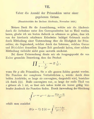
All of these great mathematicians used ideas from a chap called Bernhard Riemann who wrote a short but historic paper titled, "On the Number of Primes Less Than A Given Magnitude".

In just 10 pages he set out new ideas that have inspired generations of mathematicians even to this day. It's hard to overestimate the historic importance of his paper.

One of the new ideas Riemann introduced was the connection between the prime counting function $\pi(x)$ that we've been talking about, and a function we now call the Riemann Zeta function $\zeta(s)$. He discovered that the distribution of primes is related to the zeros of this zeta function. In fact he suggested that the zeros only occur when complex $s$ has real part $\frac{1}{2}$ and no-where else (except for trivial zeros at negative even numbers, -2, -4. -6, etc).

In concise maths, Riemann suggested:

$$ \zeta(s) = 0 \iff s = \frac{1}{2} + it$$

Sadly, he didn't prove it in his paper. And nobody has been able to prove that innocent looking statement since.

In fact this problem, the Riemann Hypothesis, is considered one of the most important mathematical unsolved problems today. It is one of the Clay Institute millennium challenges and a successful proof will attract a $1 million dollar prize.

We've talked about this important Riemann Zeta function but we haven't explained what it actually is. We'll do that next in a little more detail.

Riemann's Zeta Function

Before we dive into the Riemann Zeta function let's go back to basics and see how it came about.

Euler, one of the greatest mathematicians of all time, was interested in infinite series, that is, series that go on forever.

Here's a simple example:

$$ \sum_{n=1}^{\infty} {n} =  1 + 2 + 3 + 4 + \cdots $$

As we keep adding these ever increasing numbers, the sum gets larger and larger and larger. Loosely speaking, the sum of this series is infinity.

What about this one?

$$ \sum_{n=1}^{\infty} {\frac{1}{2n}} =  \frac{1}{1} + \frac{1}{2} + \frac{1}{4} + \frac{1}{8} + \cdots $$

We can see that numbers in this series get smaller and smaller and smaller. Adding these numbers, we can see that the sum gets closer and closer to 2. We can imagine that if we did somehow add the whole infinite series, the sum would be 2. Some people don't like that leap, and prefer to say that in the limit, as $n$ goes to infinity, the sum goes to 2. That's a perfectly fine way to think about it.

Let's look at another one:

$$ \sum_{n=1}^{\infty} {\frac{1}{n}} =  \frac{1}{1} + \frac{1}{2} + \frac{1}{3} + \frac{1}{4} + \cdots $$

Looking at this series, we can see the numbers get smaller and smaller. In fact, each number is half the previous number. Does that mean the sum of the infinite series is some finite number? It may surprise you that the answer is no. This series, called the harmonic series, does actually grow to infinity, but does so very slowly.

The lesson from that last harmonic series is that it isn't always obvious whether an infinite series converges to a finite value, or whether it diverges to infinity.

Anyway, Euler was interested in series of this form:

$$ \zeta(s) = \sum_{n=1}^{\infty} {\frac{1}{n^s}} =  \frac{1}{1^s} + \frac{1}{2^s} + \frac{1}{3^s} + \frac{1}{4^s} + \cdots $$

We can see there's a new variable $s$ which could be any number, like $s=4$ or $s=100$. For $s=2$ this series is

$$
\begin{align}
\zeta(2) = \sum_{n=1}^{\infty} {\frac{1}{n^2}} & =  \frac{1}{1^2} + \frac{1}{2^2} + \frac{1}{3^2} + \frac{1}{4^2} + \cdots \\
& =  1+ \frac{1}{4} + \frac{1}{9} + \frac{1}{16} + \cdots \\
\end{align}
$$

Different values of $s$ give different series. The general form $\zeta(s)$ is called a zeta function.

It's natural to ask whether the series created by different values of $s$ converge. Maybe they all do? Maybe none do? Maybe some of them do and some don't.

Let's see what happens when $s=1$. The series becomes $\zeta(1) = \frac{1}{1} + \frac{1}{2} + \frac{1}{3} + \frac{1}{4} + \cdots$ which is the harmonic series we saw earlier, and we know this doesn't converge.

What about $s=2$. The series becomes $\zeta(2) = \frac{1}{1} + \frac{1}{4} + \frac{1}{9} + \frac{1}{16} + \cdots$. It turns out that this series does converge, and actually converges to $\frac{\pi^2}{6}$.

Is there a way to see which values of $s$ create series that do converge? The usual simple ratio test to see if a series converges is inconclusive.

Let's get creative! Have a look at the following picture:

We can see that the area of the rectangles is always less than the area under the curve. If the rectangles have width 1 and height $\frac{1}{n^s}$, that means:

$$ \sum_{n=1}^{\infty}\frac{1}{n^s} < 1 + \int_{1}^{\infty} \frac{1}{t^s} \, dt $$

Doing that integral is easy - just as we learned at school:

$$
\begin{align}
\int_{1}^{\infty} \frac{1}{t^s} \, dt  & = \lim_{a \to \infty}  \int_{1}^{a} \frac{1}{t^s} \, dt  \\
& = \lim_{a \to \infty} \left[\frac{1}{1-s}t^{1-s}\right]_1^{a} \\
& = \lim_{a \to \infty} \frac{1}{1-s}a^{1-s}-\frac{1}{1-s} \\
\end{align}
$$

Now, we can see that as $a$ gets larger and larger towards $\infty$, the only way that expression is going to converge is if that $a^{1-s}$ doesn't grow larger and larger. That means $a$ must be raised to a negative number. That is, $1-s < 0$, or $s > 1$.

So, to summarise, if $ \zeta(s) = \sum_{n=1}^{\infty}\frac{1}{n^s} $ is always less than $ 1 + \int_{1}^{\infty} \frac{1}{t^s} \, dt $, which only converges if $s > 1$ .. we have our condition that the zeta function only converges if $s > 1$. Phew!

You can read more about this technique here [link], and I received help here [link].

Now that we know the $\zeta(s)$ function only works when $s > 1$, let's plot it.

The code to do this is really simple. We simply create an evenly spaced list of numbers, from 1.1 to 9.9, spaced every 0.1. We then calculate $\zeta(s)$ for all these values of $s$, and plot a graph. We could have hand-coded our own function to work out $\zeta(s)$ by summing, say the first 10 or 100 terms in the series, but we can use the convenience function provided by the popular mpmath library.

A python notebook showing the code is here:

• https://drive.google.com/file/d/1rlVFyv_xsyN_vFm6m0teukCRn2nFYSsV/view?usp=sharing

We can see that for large $s$ the value of $\zeta(s)$ gets smaller and smaller towards 1. That makes sense, because the fractions in the series get smaller and smaller. We can also see that as $s$ gets closer to 1, the value of $\zeta(s)$ gets bigger and bigger.

Overall, we have to admit the visualisation isn't that interesting.

Into the Complex Plane

Riemann took Euler's zeta function and explored what it looked like when the parameter $s$ is not just a whole number, or even a real number, but a complex number.

We have to ask ourselves, could this work? Does the series converge, and if so, where does does it converge and where doesn't it converge?

Previously we used an integral test to find for which real values of $s$ the zeta function converged. We arrived at an expression:

$$ \lim_{a \to \infty} a^{1-s} $$

which only converges if $s > 1$. Does this still work when s is complex? Let's set $s = x + iy$,

$$
\begin{align}
a^{1-s} & = a^{1-x-iy} \\
& = a^{1-x}a^{-iy}
\end{align}
$$

That first bit $a^{1-x}$ converges when $x>1$ which is saying that the real part of $s$ must be more than 1. That's good, it's compatible with our previous conclusion. We'd be in trouble if it wasn't!

The second bit $a^{-iy}$ can be rewritten as $e^{-iy\ln{a}}$ which has a magnitude of 1, and so doesn't effect convergence. Remember that $e^{i\theta} = \cos(\theta) + i\sin(\theta)$ which are the coordinates of a unit circle on the complex plane. As $a$ grows larger and larger, $a^{-iy}$ just orbits around a circle of radius 1.

So, the zeta function $\zeta(s)$ works when s is complex, as long as the real part of $s$ is more than 1.

This should be more interesting to visualise as the complex plane is two dimensional. The following shows a plot of the complex plane with real range 1.01 to 6.01 and imaginary range -2.5i to 2.5i. The colours represent the absolute value of $\zeta(s)$.

Of course, if we only look at the absolute value of the complex values of the feta function, we're losing information on the real and imaginary parts. So let's rerun the plot but this time base the colours on the real part of $\zeta(s)$.

And again, but with the imaginary part.

The code for creating this is plot is in a python notebook:

• https://drive.google.com/open?id=1OK9Y2w11vRS_q5o0EJV7MlLMbu512yhJ

Looking at these plots, we can see there's a lot going on around the the point (1+0i). The plot of absolute values shows that $|\zeta(s)|$ grows large at this point. We can imagine a kind of stalagmite at this point! Interestingly the plot of the real part of the zeta function shows the action shifted right a little, and the plot of the imaginary part shows action between the point (1+0i) continuing to the right. worth coming back to this to explore it further.

Is that the only point of interest? Let's zoom out to a wider viewpoint with real part ranging from 1.01 to 31.01 and imaginary part -15i to +15i. The following shows all three absolute, real and imaginary part plots.

This wider view shows us that there is interesting stuff happening at points other than (1+0i).  It looks like there might be something happening to the left of (1+14i) and (1-14i) ... but how can this be? Surely, the zeta function only exists on the complex plane where the real part if greater than 1. Hmmmm....

Let's make a contour plot to give us a different insight into the function. The lines of a contour plot try to follow similar values. The Python matplotlib has a convenient contours plot function.

Click on the following to take a closer look.

The viewport is larger with real part going from 1.01 to 41.01, and the imaginary part from -20i to +20i. The contour plots not only reveal more curious action along the left hand edge, they also give a clearer view of how the zeta function behaves near that edge.

The code for creating these contour plots is in the following python notebook:

• https://drive.google.com/open?id=1578zRA0-MUitpupFtlXm5aMbcRNc5RwX

It's instructive to combine the three kinds of plot (absolute value, real and imaginary parts) so we can see them together:

Let's now return to that question we asked earlier. Those contour lines seem to point to something that's happening off the left-hand edge, $\Re(s) = 1$. It's as if the pattern was brutally cut off before we could see it in its entirety.

Let's imagine what would happen if we continued those lines.

This is really interesting. The maths tells us that the contour lines must stop at $\Re(s) = 1$ because the zeta function doesn't converge for $s \le 1$. We can't argue with the maths. And yet, the picture suggests very strongly that the pattern does continue.

Curiouser and curiouser!

Analytic Continuation

One of several strokes of genius that Riemann had was to resolve that puzzle above.

Have a look at the following infinite series:

$$ f(x) =  1 + x + x^2 + x^3 + x^4 + x^5 + ... $$

We already know that this series only converges if each successive term doesn't increase, that is $x < 1$. What if we used a complex number $z$ instead of a plain normal number $x$?

$$ f(z) =  1 + z + z^2 + z^3 + z^4 + z^5 + ... $$

How do we decide for which $z$ this converges? If we write $z$ in the polar coordinate form $z = r \cdot e^{i\theta}$, we can see that

$$ f(z) = 1 +  r \cdot e^{i\theta} +  r^2 \cdot e^{i2\theta} +  r ^3 \cdot e^{i3\theta} + ... $$

The ratio test gives us

$$
\begin{align}
\lim_{n \to \infty} \vert \frac { r ^{n+1} \cdot e^{i(n+1)\theta}} { r^n \cdot e^{in\theta}} \vert & < 1 \\
\\
\lim_{n \to \infty} \vert  r  \cdot e^{i\theta}  \vert & < 1 \\
\\
\vert r \vert & < 1 \\
\end{align}
$$

So the series converges as long as the complex number $z$ is within the unit circle, as shown in the next picture.

Now, let's take a different perspective on that series.

$$
\begin{align}
f(z) & =  1 + z + z^2 + z^3 + z^4 + z^5 + ... \\
z \cdot (f(z) & =  z + z^2 + z^3 + z^4 + z^5 + z^6 + ... \\
1 + z \cdot (f(z) & =  1 + z + z^2 + z^3 + z^4 + z^5  + ... \\
& = f(z) \\
1 &= (1-z) \cdot f(z) \\
f(z) &= \frac{1}{1 - z} \\
\end{align}
$$

So we have a simple expression for the sum of that series. But this expression doesn't itself suggest that $\vert z \vert < 1$. It only suggests that $z \ne 1$.

What's going on ?!

One way to think about this is that $f(z) = \frac{1}{1 - z}$ is function which works over the entire complex plane, except at $z = 1$, and that the series $f(z) =  1 + z + z^2 + z^3 + z^4 + z^5 + ... $ is just a representation which works only for $\vert z \vert < 1$. In fact, it is just one of many representations. Another, slightly more complicated, representation is $f(z) = \int_0^{\infty} {e^{-t(1-z}}\,dt$ which works over $\Re(z) < 1$, which also covers the left-half plane.

What analytic continuation does is to take a representation which has a limited domain over which it works, and tries to find a different representation which works over a different domain. If we're lucky we might find the function that works everywhere, or at least the maximum possible.

There are several methods to do this analytic continuation, and they all depend on the fact that if two representations overlap, and have the same values there, then they are compatible in quite a strong sense. Actually doing the continuation is fairly heavy with algebra so we won't do it here. What we can do is get  an intuitive feel for how and why analytic continuation works.

Have a look at the following, which shows the same zone of convergence of the series representation as before.

This time we're noting that the series is in fact the Taylor expansion of $f(z) = \frac{1}{1 - z}$ about $z=0$ and the radius of converge is the distance from $z=0$ to the nearest pole, which is at $z=1$ in this example. A pole is just a point where the function isn't defined and in the limit approaches infinity. Think of pole holding up a tent cloth!

Now, what happens if we take a Taylor series expansion of the same $f(z) = \frac{1}{1 - z}$ but about a different point, $z = 1 + 0.5i$, or example.

The resultant series, which is fairly easy to work out, has a radius of convergence centred about $z = 1 + 0.5i$ and extends to the pole. In fact that circle is smaller than our previous one because the pole is closer. But notice that this new domain covers a part of the complex plane that the previous circle didn't.

We've extended the domain! And we can keep doing it ..

We can keep doing this until we cover the entire complex plane, but excluding that pole of course. This technique is especially useful if we didn't know the true function, but only series representations which have limited domains.

Can this be done with the Riemann Zeta function, which in the series form, only works for $\Re(z) > 1$. Those contour plots strongly suggested it could be. The answer is yes! In fact it can be extended to the entire complex plane, and that continuation has only one pole at $z=1$ and many zeros. We won't do it here because the algebra is heavy.

What we can do is use software like the Python mpmath library to visualise the rest of the Riemann Zeta function.

We can see the values do continue naturally from that hard boundary we have before at $\re(z) = 1$. We can also see that the values are a lot more varying in the left half of the complex plane. To the right the function seems to be very calm, boring even.

Interestingly, we can see what look like zeros of the zeta function going up the line $\Re(z) = \frac{1}{2}$. That's worth a closer look.

Let's see what a contour plots can show us.

Those zeros have become really clear. There are three things to note:

• There are zeros up the line $\Re(z) = \frac{1}{2}$
• There are zeros at every negative even number on the real line, -2, -4, -6, -8, ...
• There is one pole at 1.

For completeness, the following plots compare the real and imaginary contours. The values, which cover a very broad range, have been subjected to a natural log just to aid visualisation.

The code for these plots are online:

• colour plots: https://drive.google.com/open?id=13CLcA8at9JoHQJw7lo0sPNucCcAabtJ2
• contour plots: https://drive.google.com/open?id=18jgeJg_8fa1ka4AxoC5Ek-AKdz7ZxW0i

The following is a higher resolution plot combining the colour plot and the contours for absolute and real parts.

Zeta Zeros - $1 Million Prize!

Mathematicians have proved:

• there is only one pole in the version of the Riemann Zeta function extended to the entire complex plane
• there are zeros at $-2n$, the negative odd real numbers

But, mathematicians have not yet proved that the other, so-called non-trivial zeros, are all on the vertical line $\Re(z) = \frac{1}{2}$. 

If you can do that, or disprove it, you'll be awarded 1 million dollars.

In 1903, 15 non-trivial zeros of the Riemann Zeta function were found. By 2004, $10^{13}$ zeros were found, all on the line  $\Re(z) = \frac{1}{2}$. That looks like extremely convincing evidence - but it is still not proof.

This challenge has been open since Riemann's 1859 paper, and was part of Hilbert's 1900 collection of unsolved important problems, as well as the Clay Institute's millennial problems set out in the year 2000.

More Reading

• Nice easy-going video on visualising the Riemann Zeta function https://www.youtube.com/watch?v=sD0NjbwqlYw
• Barry Mazur "A Lecture on Primes and the Riemann Hypothesis" (video) https://www.youtube.com/watch?v=way0jAWpjZA
• One of the best explanations of the Riemann Hypothesis: https://medium.com/@JorgenVeisdal/the-riemann-hypothesis-explained-fa01c1f75d3f
• The official Clay Institute millennium challenge: http://www.claymath.org/millennium-problems/riemann-hypothesis
• English translation of Riemann's "One The Number of Primes Less Than A Given Magnitude": http://www.claymath.org/sites/default/files/ezeta.pdf
• A good overview of the Prime Number Theorem and the Riemann Hypothesis: https://thatsmaths.com/2014/02/27/the-prime-number-theorem/
• A very readable introduction to analytic continuation: http://www.mathpages.com/home/kmath649/kmath649.htm
• Another intro to analytic continuation showing other methods: https://www.colorado.edu/amath/sites/default/files/attached-files/pade_analytic_continuation.pdf
• Download the zeros of the Riemann Zeta function: http://www.dtc.umn.edu/~odlyzko/zeta_tables/